Download
1 / 21
210 likes | 294 Vues
Rachel Howe. Helioseismology with Synoptic Network Observations. Why do we need to continue observing? Why ground-based? Requirements for a new network. Synopsis. Why continue observing?. Long-term variations. Dynamics changes – rotation-rate variations Part of the puzzle for the dynamo

E N D
Rachel Howe Helioseismology withSynoptic Network Observations
Why do we need to continue observing? Why ground-based? Requirements for a new network Synopsis
Long-term variations Dynamics changes – rotation-rate variations Part of the puzzle for the dynamo Useful for “preview” of activity cycle timing
Long-term variations -- dynamics Rotation-rate variations near the tachocline
Torsional oscillation from ring-diagram analysis: MDI-GONG combo that I showed at the AGU meeting. MDI before mid-2001, GONG after. The flows are averaged in depth over 4-10 Mm. Bands of faster (or slower) rotation move toward the equator. The fast band of cycle 24 appears before there is any surface activity present. The new fast band is stronger in the northern hemisphere indicating that the activity will be stronger in this hemisphere. Courtesy of R. Komm Torsional Oscillation (local helioseismology)
Meridional Circulation Variation Temporal variation of the fitted polynomial to the meridional circulation observations at a depth of 5.8 Mm. (Bottom panel symmetrized; poleward velocities positive.) Figure 2 from Meridional Circulation During the Extended Solar Minimum: Another Component of the Torsional Oscillation? I. GonzálezHernández et al. 2010 ApJ 713 L16 doi:10.1088/2041-8205/713/1/L16
ACRIM (Woodard & Noyes 1985, 1988, Gelly, Fossat & Grec 1988) BiSON, Mark I (Palle et al. 1989, Elsworth et al. 1990) Chaplin et al. 2007 Frequency shifts with solar cycle
Normalized even-a coefficients vary as Legendre decomposition of magnetic field distribution Asphericity variations
Normalized even-a coefficients vary as Legendre decomposition of magnetic field distribution – but fit isn’t perfect; residuals correlated between GONG, MDI Asphericity variations
Long-term variations (structure) Localized GONG frequency shifts
Why ground-based? Redundancy/ease of repair -- lose one site for a few months, still get usable data
Longevity Why ground-based? BiSON – courtesy W. Chaplin
Redundancy Why ground-based?
Minimum for global: continuation of GONG classic cadence/resolution/duty cycle • For local: • > 75% duty cycle, • <0.1 deg angular drift • Overlap between sites for cross-calibration • Minimum 1-year overlap with predecessor • Improved peak fitting Basic Requirements
Work for example with AIA UV intensity has shown how mode behavior varies through the atmosphere Multi-wavelength
Power Maps 3mHz 5mHz 7mHz HMI V HMI Ic HMI Lc AIA 1700