Download
1 / 1
10 likes | 84 Vues
Statistical Analyses. Abstract. Materials and Methods. Results. Shannon- Weiner Index (SWI). Shannon- Weiner Index (SWI). Conclusions and Future Directions. Spatial Distribution of Biodiversity of Juvenile Fin Fish Mary C. Christman 1 * , Kevin Donaldson 1 , and Thomas Miller 2

E N D
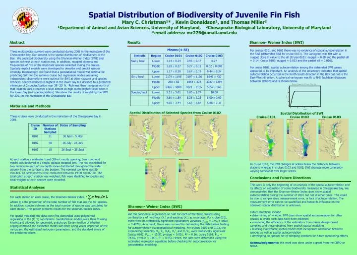
Statistical Analyses Abstract Materials and Methods Results Shannon- Weiner Index (SWI) Shannon- Weiner Index (SWI) Conclusions and Future Directions Spatial Distribution of Biodiversity of Juvenile Fin Fish Mary C. Christman1* , Kevin Donaldson1, and Thomas Miller2 1Department of Animal and Avian Sciences, University of Maryland, 2Chesapeake Biological Laboratory, University of Maryland *email address: mc276@umail.umd.edu Means (± SE) For cruises 0101 and 0103 there was no evidence of spatial autocorrelation in the SWI (detrended SWI for cruise 0103). The variogram was flat with a nugget close in value to the sill (Cruise 0101: nugget = 0.68 and the partial sill = 0.14; Cruise 0103: nugget = 0.023 and the partial sill = 0.016). For cruise 0102, spatial autocorrelation among the detrended SWI values appeared to be important. An analysis of the anisotropy indicated that spatial autocorrelation occurred in the North-South direction in the Bay but not in the East-West direction. A spherical variogram was fit to N-S Euclidean distances between stations and is shown below. Three multispecies surveys were conducted during 2001 in the mainstem of the Chesapeake Bay. Our interest is the spatial distribution of biodiversity in the Bay. We analyzed biodiversity using the Shannon-Weiner Index (SWI) and species richness at each station and, in addition, mapped biomass and frequencies of five of the important species collected during the cruises. Spatially explicit models were developed to describe and predict species diversity. Interestingly, we found that a geostatistical model was optimal for predicting SWI for the summer cruise but regression models assuming independent observations were optimal for SWI at other seasons and species richness. Species richness is highest in the lower Bay but declines to a predicted minimum of 2 species/station near 38 25 N. Richness then increases north of that location until it reaches a level almost as high as the highest level seen in the lower Bay (6-7 species/station). We show the results of modeling the SWI for 2001 in the mainstem of the Chesapeake Bay. Spatial Distribution of Selected Species from Cruise 0102 Spatial Distribution of SWI Three cruises were conducted in the mainstem of the Chesapeake Bay in 2001. Cruise 0101 Cruise 0102 Cruise 0103 At each station a midwater trawl (18-m2 mouth opening, 6-mm cod end mesh) was deployed in a single, oblique stepped tow. The net was fished for two minutes in each of ten depth zones distributed throughout the water column from the surface to the bottom. The nominal tow time was 20 minutes. All deployments were conducted between 19:00 and 07:00. The total catch at each station was weighed; fish were identified to species and total weights of each species were recorded. In cruise 0101, the SWI changes at scales below the distances between stations whereas in cruises 0102 and 0103, SWI changes more coherently varying somewhat over larger scales. • This work is only the beginning of an analysis of the spatial autocorrelation and its effects on estimation of some biodiversity measures in Chesapeake Bay. We • demonstrated that the Shannon-Weiner Index does show spatial autocorrelation during the summer of 2001 but not at other times. This could be due to sample sizes, measurement error, or lack of autocorrelation. The measurement error cannot be quantified and hence its influence on the observed spatial distribution is unknown. • Future directions include • determining of whether SWI does show spatial autocorrelation for other cruises in which such data have been collected • comparing the efficiency of the estimators from classic design-based • sampling and those obtained from explicit spatial modeling • building multivariate spatial models that incorporate correlation between species as well as spatial autocorrelation • developing an optimal set of sampling locations for future monitoring efforts • Acknowledgements: this work was done under a grant from the CBPO or NOAA. For each station on each cruise, the Shannon-Weiner index, where pi is the proportion of the total number of fish that are the ith species. In addition, species richness as the total number of species was calculated for each station. This poster presents results for the Shannon-Weiner Index. For spatial modeling the data were first detrended using polynomial regression in the (X, Y) coordinates. Geostatistical models were then fit using kriging and allowing for geometric anisotropy. Determination of whether kriging improved the estimated model was done using visual inspection of the variogram, the estimated variogram parameters, and the standard errors of the predicted values. We ran polynomial regressions on SWI for each of the three cruises using combinations of northings (X1) and eastings (X2) as covariates. For cruise 0101, there were no statistically significant explanatory variables (F7,23 = 0.97, p-value = 0.4878). As a result, there was no need for detrending the data before testing for autocorrelation via geostatistical modeling. For cruises 0102 and 0103, the explanatory variables, X1, X2, X1X2, X12, and X12X2, were statistically significant (cruise 0102: F5,42 = 10.57, p-value < 0.001, R2 = 0.56; cruise 0103: F5,9 = 34.65, p-value < 0.001, R2 = 0.95). Hence, the data were detrended using the estimated regression equations before checking for autocorrelation via geostatistical modeling.