Download
1 / 41
540 likes | 1.53k Vues
Ch 4 Fluids in Motion. Introduction. In the previous chapters we have defined some basic properties of fluids and have considered various situations involving fluids that are at rest.

E N D
Introduction In the previous chapters we have defined some basic properties of fluids and have considered various situations involving fluids that are at rest. In general, fluids have a well-known tendency to move or flow. The slightest of shear stresses will cause the fluid to move. Similarly, an appropriate imbalance of normal stresses (pressure) will cause fluid motion. In this chapter we will discuss various aspects of fluid motion without being concerned with the actual forces necessary to produce the motion. That is, we will consider the kinematics of the motion—(the velocity and acceleration of the fluid, and the description and visualization of its motion. No forces) The analysis of the specific forces necessary to produce the motion (the dynamics of the motion) will be discussed in detail in the following chapters. A wide variety of useful information can be gained from a thorough understanding of fluid kinematics. Such an understanding of how to describe and observe fluid motion is an essential step to the complete understanding of fluid dynamics.
Flow Patterns: Pathline The pathline is the line traced out by a fluid particle.
Flow Patterns: Streamline The streamline is a curve that is everywhere tangent to the local velocity vector.
Flow Patterns: Streakline It is the instantaneous locus of all fluid particles that have passed through a given point. If at point A in a flow field, a dye is injected, then the photograph of the dye streak would be a streakline. In other words, if fluid particles 1 through 4 have passed successively through point A, the shown dotted line (joining all these particles at time t) would be the streakline.
Dividing Streamline and Stagnation Point • When an object divides the flow, then the streamline that follows the flow division is called “dividing streamline”. • The point of division is called the stagnation point (since the flow is stagnant there).
Laminar and Turbulent Flow • In laminar flow, the fluid flows in layers parallel to each other. No mixing. • In turbulent flow, the velocity is fluctuating with time and a strong mixing occurs between fluid layers.
1 Dimensional Flow Not very good assumption but many practical flows could be modeled as 1 D flow Pipe flow: Function of radial position, r, only ! Duct flow: Function of axial distance, x, only !
Methods of Predicting Velocity Field • Analytical methods: • Solving a set of equations to get the velocity field. • Numerical methods: Solving the same set of equations using numerical methods. Predicted streamline pattern over theVolvo ECC prototype.
Experimental methods Pathlines of floating particles • We inject fluid markers (ink or dust) and study the streamlines, pathlines and streaklines. Smoke traces about an airfoil with a large angle of attack.
Volume Flow Rate • Flow rate (or discharge, Q) is defined as the rate at which a certain fluid volume passes through a given section in the flow stream. • V is assumed to be constant.
Volume Flow Rate, Q If the velocity is constant over the cross section, But if V is not normal to dA
Average Velocity We define the average velocity as But what is dA?
Acceleration in Cartesian and Streamline Coordinates (a) Cartesian coordinates (b) Streamline coordinates
Acceleration in Cartesian Coordinates This is a vector result whose scalar components can be written as
1D acceleration 2D acceleration 3D acceleration
Convective Acceleration Local Acceleration
Streamline Coordinates In the streamline coordinate system the flow is described in terms of one coordinate along the streamlines, denoted s, and the second coordinate normal to the streamlines, denoted n.
Acceleration in Streamline Coordinates Normal acceleration, an Tangential acceleration, at Local acceleration Convective acceleration.
Uniform Flow Patterns In the uniform flow, the velocity vector (magnitude + direction) does not change a long a streamline.The streamlines should be straight and parallel to each other.
Non-uniform Flow Patterns In figure a, the streamlines are straight but not parallel. So, a change in the velocity magnitude will occur as we move along the streamline. In figure b, the streamlines are parallel but they are not straight. So, a change in the velocity direction occurs.
System and Control Volume • A fluid system is a given quantity of matter consisting always of the same matter. • A control volume (CV) is a geometric volume defined in space and enclosed by a control surface.
Lagrangian Method There are two approaches to describe the velocity of a flowing field. • The position of a specific fluid particle traveling along a pathline is recorded with time.
Eulerian Method • The properties of fluid particle passing a given point in space are recorded with time. • The Eulerian approach is generally used to analyze fluid motion.
Control Volume Equation(Reynolds Transport Equation) This equation relates the time rate of change of a property of a system to the time rate of change of the property in a control volume plus the net efflux of the property across the control surface.
Intensive and Extensive propertiesof a System • Intensive properties are those that are independent of the mass of the system. • Extensive properties are those that are dependent on the system mass. The amount of an extensive property that a system possesses at a given instant, can be determined by adding up the amount associated with each fluid particle in the system.
Derivation of the Control Volume Equation(Reynolds Transport Equation) See also handouts
Uniform Velocity distribution If the velocity is not uniform over the cross section If the flow is steady, this term is zero
Application of Reynolds Transport Equation toConservation of Mass Principle(Integral Form of the Continuity Equation) General form of the Integral continuity equation
Continuity at a PointDifferential Form of the Continuity Equation • If the flow is steady • If the flow is also incompressible
Rotation • The rotational rate of a fluid element is the average rotational rate of two initially perpendicular sides of a fluid particle.
Vorticity The Vorticity of a fluid particle is a vector equal to twice the rotational rate of the particle. For irrotational flow:
A forced vortex is a rotational flow with concentric circular streamlines in which the fluid rotates as a solid body. A free (potential) vortex is an irrotational flow in which the velocity varies inversely as the distance from the center. Vortices
Separation • Separation in a flow occurs when the streamlines move a way from the body boundaries and a local re-circulation region occurs.