Download
1 / 52
520 likes | 737 Vues
Fluids in Motion. P M V Subbarao Associate Professor Mechanical Engineering Department IIT Delhi. An Unique Option for Many Power Generation Devices. Velocity and Flow Visualization. Primary dependent variable is fluid velocity vector V = V ( r ); where r is the position vector.

E N D
Fluids in Motion P M V Subbarao Associate Professor Mechanical Engineering Department IIT Delhi An Unique Option for Many Power Generation Devices..
Velocity and Flow Visualization • Primary dependent variable is fluid velocity vector V = V ( r ); where r is the position vector. • If V is known then pressure and forces can be determined. • Consideration of the velocity field alone is referred to as flow field kinematics in distinction from flow field dynamics (force considerations). • Fluid mechanics and especially flow kinematics is a geometric subject and if one has a good understanding of the flow geometry then one knows a great deal about the solution to a fluid mechanics problem.
Particle p at time t1 Particle p at time t2 Uniform Flow Flow Past A Turbine Blade
Velocity: Lagrangian and Eulerian Viewpoints There are two approaches to analyzing the velocity field: Lagrangian and Eulerian Lagrangian: keep track of individual fluids particles. Apply Newton’s second law for each individual particle! Say particle p is at position r1(t1) and at position r2(t2) then,
Of course the motion of one particle is insufficient to describe the flow field. So the motion of all particles must be considered simultaneously which would be a very difficult task. Also, spatial gradients are not given directly. Thus, the Lagrangian approach is only used in special circumstances.
Eularian Approach Eulerian: focus attention on a fixed point in space. In general, where, u = u(x,y,z,t), v = v(x,y,z,t), w = w(x,y,z,t)
This approach is by far the most useful since we are usually interested in the flow field in some region and not the history of individual particles. This is similar to description of A Control Volume. We need to apply newton Second law to a Control Volume.
Eularian Velocity • Velocity vector can be expressed in any coordinate system; e.g., polar or spherical coordinates. • Recall that such coordinates are called orthogonal curvilinear coordinates. • The coordinate system is selected such that it is convenient for describing the problem at hand (boundary geometry or streamlines).
Fluid Dynamics of Coal Preparation & Supply BY P M V Subbarao Associate Professor Mechanical Engineering Department I I T Delhi Aerodynamics a means of Transportation ……
Schematic of typical coal pulverized system A Inlet Duct; B Bowl Orifice; C Grinding Mill; D Transfer Duct to Exhauster; E Fan Exit Duct.
Velocity through various regions of the mill during steady operation
Cyclone-type classifier. Axial and radial gas velocity components
Centrifugal Classifiers • The same principles that govern the design of gas-solid separators, e.g. cyclones, apply to the design of classifiers. • Solid separator types have been used preferentially as classifiers in mill circuits: • centrifugal cyclone-type and gas path deflection, or • louver-type classifiers. • The distributions of the radial and axial gas velocity in an experimental cyclone precipitator are shown in Figures. • The flow pattern is further characterized by theoretical distributions of the tangential velocity and pressure, the paths of elements of fluid per unit time, and by the streamlines in the exit tube of the cyclone.
Particle Size Distribution--Pulverized-Coal Classifiers • The pulverized-coal classifier has the task of making a clean cut in the pulverized-coal size distribution: • returning the oversize particles to the mill for further grinding • but allowing the "ready to burn" pulverized coal to be transported to the burner. • The mill's performance, its safety and also the efficiency of combustion depend on a sufficiently selective operation of the mill classifier.
Mill Pressure Drop • The pressure loss coefficients for the pulverized-coal system elements are not well established. • The load performance is very sensitive to small variations in pressure loss coefficient. Correlation of pressure loss coefficient with Reynolds number through the mill section of an exhauster-type mill.
Volume Rate of Flow (flow rate, discharge) • Cross-sectional area oriented normal to velocity vector (simple case where V . A).
Acceleration • The acceleration of a fluid particle is the rate of change of its velocity. • In the Lagrangian approach the velocity of a fluid particle is a function of time only since we have described its motion in terms of its position vector.
In the Eulerian approach the velocity is a function of both space and time; consequently, x,y,z are f(t) since we must follow the total derivative approach in evaluating du/dt.
Similarly for ay & az, In vector notation this can be written concisely
Control Volume • In fluid mechanics we are usually interested in a region of space, i.e, control volume and not particular systems. • Therefore, we need to transform GDE’s from a system to a control volume. • This is accomplished through the use of Reynolds Transport Theorem. • Actually derived in thermodynamics for CV forms of continuity and 1st and 2nd laws.
Flowing Fluid Through A CV • A typical control volume for flow in an funnel-shaped pipe is bounded by the pipe wall and the broken lines. • At time t0, all the fluid (control mass) is inside the control volume.
The fluid that was in the control volume at time t0 will be seen at time t0 +dt as: .
The control volume at time t0 +dt . The control mass at time t0 +dt . The differences between the fluid (control mass) and the control volume at time t0 +dt .
II I • Consider a system and a control volume (C.V.) as follows: • the system occupies region I and C.V. (region II) at time t0. • Fluid particles of region – I are trying to enter C.V. (II) at time t0. III II • the same system occupies regions (II+III) at t0 + dt • Fluid particles of I will enter CV-II in a time dt. • Few more fluid particles which belong to CV – II at t0 will occupy III at time t0 + dt.
III II At time t0+dt II I At time t0 The control volume may move as time passes. III has left CV at time t0+dt I is trying to enter CV at time t0
Reynolds' Transport Theorem • Consider a fluid scalar property b which is the amount of this property per unit mass of fluid. • For example, b might be a thermodynamic property, such as the internal energy unit mass, or the electric charge per unit mass of fluid. • The laws of physics are expressed as applying to a fixed mass of material. • But most of the real devices are control volumes. • The total amount of the property b inside the material volume M , designated by B, may be found by integrating the property per unit volume, M ,over the material volume :
Conservation of B • total rate of change of any extensive property B of a system(C.M.) occupying a control volume C.V. at time t is equal to the sum of • a) the temporal rate of change of B within the C.V. • b) the net flux of B through the control surface C.S. that surrounds the C.V. • The change of property B of system (C.M.) during Dt is add and subtract
The above mentioned change has occurred over a time dt, therefore Time averaged change in BCMis
For and infinitesimal time duration • The rate of change of property B of the system.
Conservation of Mass • Let b=1, the B = mass of the system, m. The rate of change of mass in a control mass should be zero.
Conservation of Momentum • Let b=V, the B = momentum of the system, mV. The rate of change of momentum for a control mass should be equal to resultant external force.
Conservation of Energy • Let b=e, the B = Energy of the system, mV. The rate of change of energy of a control mass should be equal to difference of work and heat transfers.
First Law for A Control Volume • Conservation of mass: • Conservation of energy:
Complex Flows in Power Generating Equipment Separation, Vortices, and Turbulence
Turbulent Flow Turbulent flow: fuller profile due to turbulent mixing extremely complex fluid motion that defies closed form analysis. • Turbulent flow is the most important area of power generation fluid flows. • The most important nondimensional number for describing fluid motion is the Reynolds number
Internal vs. External Flows • Internal flows = completely wall bounded; • Usually requires viscous analysis, except near entrance. • External flows = unbounded; i.e., at some distance from body or wall flow is uniform. • External Flow exhibits flow-field regions such that both inviscid and viscous analysis can be used depending on the body shape and Re.