Download
1 / 47
480 likes | 673 Vues
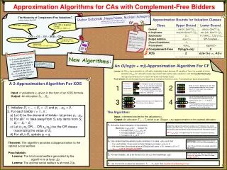
Approximation Algorithms for Combinatorial Auctions with Complement-Free Bidders. Speaker: Michael Schapira Joint work with Shahar Dobzinski & Noam Nisan. Talk Structure. Combinatorial Auctions Log(m)-approximation for CF auctions

E N D
Approximation Algorithms forCombinatorial Auctions with Complement-Free Bidders Speaker: Michael Schapira Joint work with Shahar Dobzinski & Noam Nisan
Talk Structure • Combinatorial Auctions • Log(m)-approximation for CF auctions • An incentive compatible O(m1/2)-approximation of CF auctions using value queries. • 2-approximation for XOS auctions • A lower bound of e/(e-1)-e for XOS auctions
Combinatorial Auctions • A set M of items for sale. |M|=m. • n bidders, each bidder i has a valuation function vi:2M->R+. Common assumptions: • Normalization: vi()=0 • Free disposal: ST vi(T) ≥ vi(S) • Goal: find a partition S1,…,Sn such that social welfare Svi(Si) is maximized
Combinatorial Auctions • Problem 1: finding an optimal allocation is NP-hard. • Problem 2: valuation length is exponential in m. • Problem 3: how can we be certain that the bidders do not lie ? (incentive compatibility)
Combinatorial Auctions • We are interested in algorithms that based on the reported valuations {vi }i output an allocation which is an approximation to the optimal social welfare. • We require the algorithms to be polynomial in m and n. That is, the algorithms must run in sub-linear (polylogarithmic) time. • We explore the achievable approximation factors.
Access Models How can we access the input ? • One possibility: bidding languages. • The “black box” approach: each bidder is represented by an oracle which can answer certain queries.
Access Models • Common types of queries: • Value: given a bundle S, return v(S). • Demand: given a vector of prices (p1,…, pm) return the bundle S that maximizes v(S)-SjSpj. • General: any possible type of query (the comunication model). • Demand queries are strictly more powerful than value queries (Blumrosen-Nisan, Dobzinski-Schapira)
Known Results • Finding an optimal solution requires exponential communication. Nisan-Segal • Finding an O(m1/2-e)-approximation requires exponential communication. Nisan-Segal. (this result holds for every possible type of oracle) • Using demand oracles, a matching upper bound of O(m1/2) exists (Blumrosen-Nisan). • Better results might be obtained by restricting the classes of valuations.
The Hierarchy of CF Valuations Lehmann, Lehmann, Nisan OXS GS SM XOSCF • Complement-Free: v(ST) ≤ v(S) + v(T). • XOS: XOR of ORs of singletons • Example: (A:2 OR B:2) XOR (A:3) • Submodular: v(ST) + v(ST) ≤ v(S) + v(T). • 2-approximation by LLN. • GS: (Gross) Substitutes, OXS: OR of XORs of singletons • Solvable in polynomial time (LP and Maximum Weighted Matching respectively)
Talk Structure • Combinatorial Auctions • Log(m)-approximation for CF auctions • An incentive compatible O(m1/2)-approximation CF auctions using value queries. • 2-approximation for XOS auctions • A lower bound of e/(e-1)-e for XOS auctions
Intuition • We will allow the auctioneer to allocate k duplicates from each item. • Each bidder is still interested in at most one copy of each item (so valuations are kept the same). • Using the assumption that all valuations are CF, we will find an approximation to the original auction, based on the k-duplicates allocation.
The Algorithm – Step 1 • Solve the linear relaxation of the problem: Maximize: Si,Sxi,Svi(S) Subject To: • For each item j: Si,S|jSxi,S ≤ 1 • For each bidder i: SSxi,S ≤ 1 • For each i,S: xi,S ≥ 0 • Despite the exponential number of variables, the LP relaxation may still be solved in polynomial time using demand oracles.(Nisan-Segal). • OPT*=Si,Sxi,Svi(S)is an upper bound for the value of the optimal integral allocation.
The Algorithm – Step 2 • Use randomized rounding to build a “pre-allocation” S1,..,Sn: • Each item j appears at most k=O(log(m)) times in {Si}i. • Sivi(Si) ≥ OPT*/2. • Randomized Rounding: For each bidder i, let Si be the bundle S with probability xi,S, and the empty set with probability 1-SSxi,S. • The expected value of vi(Si) is SSxi,Svi(S) • We use the Chernoff bound to show that such “pre-allocation” is built with high probability.
The Algorithm – Step 3 • For each bidder i, partition Si into a disjoint union Si = Si1.. Sik such that for each1≤i<i’≤ n, 1≤t≤t’≤ k, SitSi’t’=.
A B D The Algorithm – Step 3 • For each bidder i, partition Si into a disjoint union Si = Si1.. Sik such that for each1≤i<i’≤ n, 1≤t≤t’≤ k, SitSi’t’=.
A B D The Algorithm – Step 3 • For each bidder i, partition Si into a disjoint union Si = Si1.. Sik such that for each1≤i<i’≤ n, 1≤t≤t’≤ k, SitSi’t’=. S11 = {A,B,D}
A D A B C D E The Algorithm – Step 3 • For each bidder i, partition Si into a disjoint union Si = Si1.. Sik such that for each1≤i<i’≤ n, 1≤t≤t’≤ k, SitSi’t’=.
A D C E The Algorithm – Step 3 • For each bidder i, partition Si into a disjoint union Si = Si1.. Sik such that for each1≤i<i’≤ n, 1≤t≤t’≤ k, SitSi’t’=. S22 = {A,D} S21 = {C,E}
A A C D E A B C D E The Algorithm – Step 3 • For each bidder i, partition Si into a disjoint union Si = Si1.. Sik such that for each1≤i<i’≤ n, 1≤t≤t’≤ k, SitSi’t’=.
A C E The Algorithm – Step 3 • For each bidder i, partition Si into a disjoint union Si = Si1.. Sik such that for each1≤i<i’≤ n, 1≤t≤t’≤ k, SitSi’t’=. S32 = {C,E} S33 = {A}
A D A B C D E A B C D E The Algorithm – Step 3 • For each bidder i, partition Si into a disjoint union Si = Si1.. Sik such that for each1≤i<i’≤ n, 1≤t≤t’≤ k, SitSi’t’=.
A B C D E A B C D E A B C D E The Algorithm – Step 3 • For each bidder i, partition Si into a disjoint union Si = Si1.. Sik such that for each1≤i<i’≤ n, 1≤t≤t’≤ k, SitSi’t’=.
A B C D E A B C D E A B C D E The Algorithm – Step 4 • Find the t maximizes Sivi(Sit) • Return the allocation (S1t,...,Snt). • All valuations are CF so: StSivi(Sit) = SiStvi(Sit) ≥ Sivi(Si) ≥ OPT*/2 For the t that maximizesSivi(Sit), it holds that: Sivi(Sit) ≥ (Sivi(Si))/k ≥ OPT*/2k = OPT*/O(log(m)).
A Communication Lower Bound of 2-e for CF Valuations Theorem: Exponential communication is required for approximating the optimal allocation among CF bidders to any factor less than 2. Proof: A simple reduction from the general case.
Talk Structure • Combinatorial Auctions • Log(m)-approximation for CF auctions • An incentive compatible O(m1/2)-approximation of CF auctions using value queries. • 2-approximation for XOS auctions • A lower bound of e/(e-1)-e for XOS auctions
Incentive Compatibility & VCG Prices • We want an algorithm that is truthful (incentive compatible). I.e. we require that the dominant strategy of each of the bidders would be to reveal true information. • VCG is the only general technique known for making auctions incentive compatible (if bidders are not single-minded): • Each bidder i pays: Sk≠ivk(O-i) - Sk≠ivk(Oi) Oi is the optimal allocation, O-i the optimal allocation of the auction without the i’th bidder.
Incentive Compatibility & VCG Prices • Problem: VCG requires an optimal allocation! • Finding an optimal allocation requires exponential communication and is computationally intractable. • Approximations do not suffice (Nisan-Ronen).
VCG on a Subset of the Range • Our solution: limit the set of possible allocations. • We will let each bidder to get at most one item, or we’ll allocate all items to a single bidder. • Optimal solution in the set can be found in polynomial time VCG prices can be computed incentive compatibility. • We still need to prove that we achieve an approximation.
The Algorithm • Ask each bidder i for vi(M), and for vi(j), for each item j. (We have used only value queries) • Construct a bipartite graph and find the maximum weighted matching P. • can be done in polynomial time (Tarjan). Bidders Items 1 v1(A) A 2 B 3 v3(B)
The Algorithm (Cont.) • Let i be the bidder that maximizes vi(M). • If vi(M)>|P| • Allocate all items to i. • else • Allocate according to P. • Let each bidder pay his VCG price (in respect to the restricted set).
Proof of the Approximation Ratio Theorem: If all valuations are CF, the algorithm provides an O(m1/2)-approximation. Proof: Let OPT=(T1,..,Tk,Q1,...,Ql), where for each Ti, |Ti|>m1/2, and for each Qi, |Qi|≤m1/2. |OPT|= Sivi(Ti) + Sivi(Qi) • Case 1: Sivi(Ti) > Sivi(Qi) • (“large” bundles contribute most of the social welfare) • Sivi(Ti) > |OPT|/2 • At most m1/2 bidders get at least m1/2 items in OPT. • For the bidder i the bidder i that maximizes vi(M), vi(M) > |OPT|/2m1/2. • Case 2:Sivi(Qi) ≥ Sivi(Ti) • (“small” bundles contribute most of the social welfare) • Sivi(Qi) ≥ |OPT|/2 • For each bidder i, there is an item ci, such that: vi(ci) > vi(Qi) / m1/2. • (The CF property ensures that the sum of the values is larger than the value of the whole bundle) • {ci}i is an allocation which assigns at most one item to each bidder: |P|≥Sivi(ci) ≥ |OPT|/2m1/2.
Talk Structure • Combinatorial Auctions • Log(m)-approximation for CF auctions • An incentive compatible O(m1/2)-approximation CF auction • 2-approximation for XOS auctions • A lower bound of e/(e-1)-e for XOS auctions
Definition of XOS • XOS: XOR of ORs of Singletons. • Singleton valuation (x:p) • v(S) = p xS 0 otherwise • Example: (A:2 OR B:2) XOR (A:3)
XOS Properties • The strongest bidding language syntactically restricted to represent only complement-free valuations. • Can describe all submodular valuations (and also some non-submodular valuations) • Can describe interesting NPC problems (Max-k-Cover, SAT).
Supporting Prices Definition: p1,…,pm supports the bundle S in v if: • v(S) = SjSpj • v(T) ≥ SjTpjfor all T S Claim: a valuation is XOS iff every bundle S has supporting prices. Proof: • There is a clause that maximizes the value of a bundle S. The prices in this clause are the supporting prices. • Take the prices of each bundle, and build a clause.
Algorithm-Example • Items: {A, B, C, D, E}. 3 bidders. • Price vector: p0=(0,0,0,0,0) v1: (A:1 OR B:1 OR C:1) XOR (C:2)Bidder 1 gets his demand: {A,B,C}.
Algorithm-Example • Items: {A, B, C, D, E}. 3 bidders. • Price vector: p0=(0,0,0,0,0) v1: (A:1 OR B:1 OR C:1) XOR (C:2)Bidder 1 gets his demand: {A,B,C}. • Price vector: p1=(1,1,1,0,0) v2: (A:1 OR B:1 OR C:9) XOR (D:2 OR E:2)Bidder 2 gets his demand: {C}
Algorithm-Example • Items: {A, B, C, D, E}. 3 bidders. • Price vector: p0=(0,0,0,0,0) v1: (A:1 OR B:1 OR C:1) XOR (C:2)Bidder 1 gets his demand: {A,B,C}. • Price vector: p1=(1,1,1,0,0) v2: (A:1 OR B:1 OR C:9) XOR (D:2 OR E:2)Bidder 2 gets his demand: {C} • Price vector: p2=(1,1,9,0,0) v3: (C:10 OR D:1 OR E:2)Bidder 3 gets his demand: {C,D,E} • Final allocation: {A,B} to bidder 1, {C,D,E} to bidder 3.
The Algorithm • Input: n bidders, for each we are given a demand oracle and a supporting prices oracle. • Init: p1=…=pm=0. • For each bidder i=1..n • Let Si be the demand of the i’th bidder at prices p1,…,pm. • For all i’ < i take away from Si’ any items from Si. • Let q1,…,qm be the supporting prices for Si in vi. • For all j Si update pj = qj.
Proof • To prove the approximation ratio, we will need these two simple lemmas: Lemma: The total social welfare generated by the algorithm is at least Spj. Lemma: The optimal social welfare is at most 2Spj.
Proof – Lemma 1 Lemma: The total social welfare generated by the algorithm is at least Spj. Proof: • Each bidder i got a bundle Ti at stage i. • At the end of the algorithm, he holds Ai Ti. • The supporting prices guarantee that: vi(Ai) ≥ SjAipj
Proof – Lemma 2 Lemma:The optimal social welfare is at most 2Spj. Proof: • Let O1,...,On be the optimal allocation. Let pi,j be the price of the j’th item at the i’th stage. • Each bidder i ask for the bundle that maximizes his demand at the i’th stage: vi(Oi)-SjOi pi,j ≤ Sj pi,j – Sj p(i-1),j • Since the prices are non-decreasing: vi (Oi )-SjOi pn,j ≤ Sj pi,j – Sj p(i-1),j • Summing up on both sides: Si vi(Oi )-SiSjOi pn,j≤Si (Sj pi,j –Sjp(i-1),j) Si vi(Oi )-Sj pn,j≤Sj pn,j Si vi(Oi ) ≤ 2Sj pn,j
Talk Structure • Combinatorial Auctions • Log(m)-approximation for CF auctions • An incentive compatible O(m1/2)-approximation of CF auctions using value queries. • 2-approximation for XOS auctions • A lower bound of e/(e-1)-e for XOS auctions
XOS Lower Bounds: • We show two lower bounds: • A communication lower bound of e/(e-1)-e for the “black box” approach. • An NP-Hardness result of e/(e-1)-e for the case that the input is given in XOS format (bidding language). • We now prove the second of these results.
Max-k-Cover • We will show a polynomial time reduction from Max-k-Cover. • Max-k-Cover definition: • Input: a set of |M|=m items, t subsets Si M, an integer k. • Goal: Find k subsets such that the number of items in their union, |Si|, is maximized. • Theorem: approximating Max-k-Cover within a factor of e/(e-1) is NP-hard (Feige).
The Reduction Max-k-Cover Instance XOS Auction with k bidders v1: (A:1 OR D:1) XOR (C:1 OR F:1) XOR (D:1 OR E:1 OR F:1) • Every solution to Max-k-Cover implies an allocation with the same value. • Every allocation implies a solution to Max-k-Cover with at least that value. • Same approximation lower bound. • A matching communication lower bound exists. A B C D E F vk: (A:1 OR D:1) XOR (C:1 OR F:1) XOR (D:1 OR E:1 OR F:1)