Download

1 / 61
620 likes | 960 Vues
Lecture 4. Short Read Alignment. The Chinese University of Hong Kong CSCI3220 Algorithms for Bioinformatics. Lecture outline. Massively parallel sequencing and short reads The short read alignment problem Suffix trie/tree/array Burrows-Wheeler Transform (BWT). Part 1.

E N D
Lecture 4. Short Read Alignment The Chinese University of Hong Kong CSCI3220 Algorithms for Bioinformatics
Lecture outline • Massively parallel sequencing and short reads • The short read alignment problem • Suffix trie/tree/array • Burrows-Wheeler Transform (BWT) CSCI3220 Algorithms for Bioinformatics | Kevin Yip-cse-cuhk | Fall 2014
Part 1 Massively Parallel Sequencing and Short Reads
DNA sequencing • DNA sequencing is the experimental procedures to find out the exact text string of a DNA sequence • Input: Multiple copies of an unknown DNA (biological) sequence • Blood sample of a patient • Some cultured bacteria • A worm • ... • Output: (Text) sequences of fragments of the DNA sequence CSCI3220 Algorithms for Bioinformatics | Kevin Yip-cse-cuhk | Fall 2014
Illustration Multiple copies of an unknown DNA biological sequence TACCAGCGGACCGCTGAC TACCAGCGGACCGCTGAC TACCAGCGGACCGCTGAC Breaking down into fragments Sequencing Text sequences of fragments TACCAG GGACCG GAC CGCTGAC TACCAG CTGAC TACCAGC CGGAC CGCT CGGAC CSCI3220 Algorithms for Bioinformatics | Kevin Yip-cse-cuhk | Fall 2014
Sequencing by synthesis • Use one strand as template, synthesize the other strand • Different ways to detect what base is added: • Give a different color for each type of nucleotide • Supply only one type of nucleotide at a time, and see if some signals (e.g., light) can be detected • Stop whenever a certain nucleotide is added. Then deduce the nucleotide by DNA lengths • Can only handle up to a certain length of DNA CSCI3220 Algorithms for Bioinformatics | Kevin Yip-cse-cuhk | Fall 2014
Sequencing by synthesis Image credit: Illumina CSCI3220 Algorithms for Bioinformatics | Kevin Yip-cse-cuhk | Fall 2014
Massively parallel sequencing (MPS) • Sequencing many short fragments in parallel • Also called “next-generation” or “deep” sequencing Image credit: Metzker, Nature Reviews Genetics 11:31-46, (2010); Azco Biotech CSCI3220 Algorithms for Bioinformatics | Kevin Yip-cse-cuhk | Fall 2014
Shotgun sequencing • Breaking down the long DNA sequence into multiple fragments due to the experimental limitation Whole genome shotgun Hierarchical approach: slightly easier to get back the original sequence Image credit: Jennifier et al., Biological Procedures Online 11(1):52-78, (2009) CSCI3220 Algorithms for Bioinformatics | Kevin Yip-cse-cuhk | Fall 2014
Short reads • The output of MPS is a list of short sequences • Each is called a read • Example: ACA, ATA, ATA, ATT, TAG, TAT, TTC • Some properties of current MPS reads: • About 100-200 nucleotides long (very short as compared to the human genome) • May overlap, since multiple copies of the original DNA are sequenced • Millions or even billions of reads from one experiment • The DNA sample may contain variations due to heterozygosity, somatic mutations and mixed population of cells • May also have contamination and sequencing errors CSCI3220 Algorithms for Bioinformatics | Kevin Yip-cse-cuhk | Fall 2014
Computational problems • Two main computational problems • Sequence alignment (this lecture): • Given a reference sequence s of length n, how to find out the position of each read r of length m in the reference? • Example situations: • Sequencing the DNA in a cancer sample – The sequence of normal human DNA can serve as a reference • Sequencing the DNA of a strain of a bacteria – The sequence of other strains of the bacteria can serve as a reference • Sequence assembly (next lecture): • Is it possible to assemble the short reads back to the original DNA? CSCI3220 Algorithms for Bioinformatics | Kevin Yip-cse-cuhk | Fall 2014
Short read alignment • Example: • Original sequence: s=TATACATTAG • Short reads:ACA, ATA, ATA, ATT, TAG, TAT, TTC • Alignment:TATACATTAG ACA ATA ATA ATT TAGTAT TTC Variation or error Image source: http://img1.etsystatic.com/000/0/6103070/il_fullxfull.203233493.jpg CSCI3220 Algorithms for Bioinformatics | Kevin Yip-cse-cuhk | Fall 2014
Short read alignment • Basically a local alignment problem, but need to align millions or billions of short sequences with a very long reference sequence, expecting almost exact matches • Need to build indexes on reads or reference • Once the indexes are built, the searching time should depend only on the size of searching results (number of hits and their locations), not the length of the reference • We will mainly study methods for exact matches CSCI3220 Algorithms for Bioinformatics | Kevin Yip-cse-cuhk | Fall 2014
Indices • Main considerations: • Space requirement • Time requirement for building index • Time requirement for searching • Main approaches: • Hash-table-based (Similar to FASTA and BLAST) • BFAST, ELAND, MAQ, MOSAIK, SHRiMP, SOAP, ZOOM, ... • Suffix-tree or Burrows-Wheeler-Transform-based • Bowtie, BWA, SOAP2, ... CSCI3220 Algorithms for Bioinformatics | Kevin Yip-cse-cuhk | Fall 2014
Hashing (revision) • Recall how k-mers of a sequence are put into a table • s= TATACATTAG 1234567890 0 1 • If we want to know whether a particular k-mer appears in this sequence, we need to know which row represents this k-mer • How? CSCI3220 Algorithms for Bioinformatics | Kevin Yip-cse-cuhk | Fall 2014
Scheme 1 • Store only the k-mers that exist in the sequence. One k-mer per table entry. • Finding if a k-mer is in the table: binary search • Index space: O(max(2k, n)) • Index building time: O(k2k+n) • Index searching time: O(k) CSCI3220 Algorithms for Bioinformatics | Kevin Yip-cse-cuhk | Fall 2014
Scheme 2 • Have one entry for every possible k-mer, no matter they exist in the sequence or not • Finding if a k-mer is in the table: Direct calculation of row number • E.g., for CT, the row number is 1*4+3+1 = 8 • Index space: O(max(2k, n)) • Index building time: O(n) • Index searching time: O(1) CSCI3220 Algorithms for Bioinformatics | Kevin Yip-cse-cuhk | Fall 2014
Scheme 3 • Use a function to map (“hash”) each k-mer into a small number • Finding if a k-mer is in the table: Compute hash value, then check the k-mers in the entry • For example, row number equals the number of A’s in the k-mer plus one • Index space: Depending on hash function, usually O(n) • Index building time: Depending on how different k-mers are stored in the same entry, can be O(n) • Index searching time: Can be same as Scheme 1 if all k-mers are hashed to the same entry. Much faster if k-mers are uniformly hashed to all entries CSCI3220 Algorithms for Bioinformatics | Kevin Yip-cse-cuhk | Fall 2014
Hashing • In general, these schemes all have to face the same two problems • Some allocated space would be wasted if the k-mers do not appear in the sequence • Collisions could occur • A typical tradeoff between space and time • One cause of the problem: The hash function has no knowledge about the sequence • We now study some data structures that make use of information about the sequence CSCI3220 Algorithms for Bioinformatics | Kevin Yip-cse-cuhk | Fall 2014
Part 2 Suffix Trie/Tree/Array
Suffixes • Given a sequence s[1..n], a suffix is either a sub-sequence s[i..n] for any i between 1 and n, or the empty string (which is sometimes represented by s[n+1..n]) • Example: s[1..10]=TATACATTAG • Suffixes: • s[1..10] TATACATTAG • s[2..10] ATACATTAG • s[3..10] TACATTAG • s[4..10] ACATTAG • s[5..10] CATTAG • s[6..10] ATTAG • s[7..10] TTAG • s[8..10] TAG • s[9..10] AG • s[10..10] G • Empty string CSCI3220 Algorithms for Bioinformatics | Kevin Yip-cse-cuhk | Fall 2014
Suffixes with end symbol • To show the empty string and to mark where the sequence ends, we will use the symbol $ to indicate the end of a sequence, and define s[n+1] to be $ • Example: s[1..11]=TATACATTAG$ • Suffixes: • s[1..11] TATACATTAG$ • s[2..11] ATACATTAG$ • s[3..11] TACATTAG$ • s[4..11] ACATTAG$ • s[5..11] CATTAG$ • s[6..11] ATTAG$ • s[7..11] TTAG$ • s[8..11] TAG$ • s[9..11] AG$ • s[10..11] G$ • s[11..11] $ CSCI3220 Algorithms for Bioinformatics | Kevin Yip-cse-cuhk | Fall 2014
Subsequence and suffixes • Important concept: Every subsequence of s is a prefix of a suffix of s • Example: • s=TATACATTAG$ • The subsequenceACATis a prefix of the suffix s[4..11]=ACATTAG$ • Therefore, finding whether a short read appears in a reference sequence is equivalent to checking whether the short read is a prefix of a suffix of the reference • To facilitate the searching of subsequences, we can put the suffixes into a tree • Suffixes: • TATACATTAG$ • ATACATTAG$ • TACATTAG$ • ACATTAG$ • CATTAG$ • ATTAG$ • TTAG$ • TAG$ • AG$ • G$ • $ CSCI3220 Algorithms for Bioinformatics | Kevin Yip-cse-cuhk | Fall 2014
Suffix trie • Tree: • A set of nodes • A set of edges, each connecting two nodes • No cycles • Suffix trie of sequence s: • A rooted tree • Every edge is labeled with one character from s • Sibling nodes are ordered alphabetically, with the end-of-sequence character $ ordered before all other characters, i.e., $ < A < C < G < T • Every path from the root to a leaf represents a suffix of s • Every suffix of s is represented by a path from the root to a leaf • Suffixes can share edges for their common prefixes CSCI3220 Algorithms for Bioinformatics | Kevin Yip-cse-cuhk | Fall 2014
Suffix trie • s=TATACATTAG$ • Suffixes:TATACATTAG$ ATACATTAG$ TACATTAG$ ACATTAG$ CATTAG$ ATTAG$ TTAG$ TAG$ AG$ G$ $ $ A C G T C G T A $ A T A $ A T T C G T A T C A T A $ A G T A G A T C $ A T $ G T A G T $ A T $ A G T G $ A $ G $ CSCI3220 Algorithms for Bioinformatics | Kevin Yip-cse-cuhk | Fall 2014
Suffix trie • s=TATACATTAG$ • To search for a length-msubsequence, simply follow the path from the root until • The subsequence is found (the subsequence appears in s), e.g., ACAT OR • You cannot go any further (the subsequence does not appear in s), e.g., CATC • Both cases take O(m) time – independent of n • Since each layer has no more than 5 nodes • A suffix trie can be constructed in time proportional to its size • Worst case O(n2) nodes $ A C G T C G T A $ A T A $ A T T C G T A T C A T A $ A G T A G A T C $ A T $ G T A G T $ A T $ A G T G $ A $ G $ CSCI3220 Algorithms for Bioinformatics | Kevin Yip-cse-cuhk | Fall 2014
Suffix tree • A suffix tree is a compact form of a suffix trie, where non-branching paths are collapsed to a single edge $ A CATTAG$ G$ T $ A C G T C G T A $ A T A $ A T T C G T A T C A T A $ A G CATTAG$ G$ T A TAG$ T A G A T C $ A T $ G T A G T $ A T $ A G T G $ A ACATTAG$ TAG$ CATTAG$ G$ TACATTAG$ $ G Suffix trie Suffix tree $ CSCI3220 Algorithms for Bioinformatics | Kevin Yip-cse-cuhk | Fall 2014
Suffix tree • The tree has no more than 2nnodes. Why? Hint: Property of binary trees • The tree can be constructed in O(n) time • We do not go into details • How much space per node? • No need to store the long edge labels as strings in the tree. Can use pointers to the original sequence s. $ A CATTAG$ G$ T CATTAG$ G$ T A TAG$ ACATTAG$ TAG$ CATTAG$ G$ TACATTAG$ CSCI3220 Algorithms for Bioinformatics | Kevin Yip-cse-cuhk | Fall 2014
Suffix tree • The tree has no more than 2nnodes. Why? Hint: Property of binary trees • The tree can be constructed in O(n) time • We do not go into details • How much space per node? • No need to store the long edge labels as strings in the tree. Can use pointers to the original sequence s. • Constant space per node • O(n) space for the whole tree 11-11: $ 2-2: A 5-11: CATTAG$ 10-11: G$ 1-1: T 5-11: CATTAG$ 10-11: G$ 3-3: T 2-2: A 8-11: TAG$ 4-11: ACATTAG$ 8-11: TAG$ 5-11: CATTAG$ 10-11: G$ 3-11: TACATTAG$ CSCI3220 Algorithms for Bioinformatics | Kevin Yip-cse-cuhk | Fall 2014
Some limitations • While suffix tree is already quite space- and time-efficient, it also has some limitations: • Some construction algorithms are quite complex • The total space needed is usually 20n bytes or more for a sequence of length n due to overheads originated from the tree structure and position indices • Think about the length of the human genome and the maximum amount of memory for a 32-bit machine • An alternative data structure: suffix array CSCI3220 Algorithms for Bioinformatics | Kevin Yip-cse-cuhk | Fall 2014
Suffix array • An array storing the original locations of the suffixes when they are sorted in lexicographic order • s=TATACATTAG$ Before sorting: After sorting: The suffix array CSCI3220 Algorithms for Bioinformatics | Kevin Yip-cse-cuhk | Fall 2014
Using a suffix array • Recall that a subsequence of s is also a prefix of a suffix of s, therefore • Finding a subsequence can be done by a binary search on the suffix array • All occurrences of the subsequence in s must be located on adjacent rows • Example: Searching for the subsequence AT s[9]=A? Yes s[9+1]=T? No. s[9+1]=G<T s[2]=A? Yes s[2+1]=T? Yes AT found in s! s[5]=A? No. s[5]=C>A Straight-forward use of suffix array requires O(mlog n) time Can improve to O(m) time by using extended suffix array – We don’t study here CSCI3220 Algorithms for Bioinformatics | Kevin Yip-cse-cuhk | Fall 2014
Time and space requirements • A suffix array can be constructed in O(n) time • Details not discussed here • If each position is stored as an integer, and each integer takes 4 bytes, the whole suffix array needs 4n bytes • For large n, we cannot assume 4 bytes is sufficient, but each index takes log nbits. The total size is thus O(nlog n) • Already quite good. Can we do even better?Goal: O(n log ||), where is the alphabet • For DNA, ||=|{A, C, G, T}| = 4 << n • Methods: • Compressed suffix arrays (not discussed here) • Burrows-Wheeler Transform (our next topic) CSCI3220 Algorithms for Bioinformatics | Kevin Yip-cse-cuhk | Fall 2014
Part 3 Burrows-Wheeler Transform
Burrows-Wheeler Transform (BWT) • Proposed by Michael Burrows and David Wheeler in 1994. • A very compact structure that can be used for text search • Input: sequence s • Conceptual* method: • Find all rotations of s and put them in a matrix • Sort the rows of the matrix in lexicographic order • Output the sequence in the last column, b *: In this lecture, whenever you see a method described as “conceptual”, it means it is used to illustrate some key ideas, but is usually too slow or too memory-demanding and we will discuss better alternative methods. CSCI3220 Algorithms for Bioinformatics | Kevin Yip-cse-cuhk | Fall 2014
Rotations and transformed string • Input: s=TATACATTAG$ • Output: b=GTTTCAAAT$A Rotations: TATACATTAG$ ATACATTAG$T TACATTAG$TA ACATTAG$TAT CATTAG$TATA ATTAG$TATAC TTAG$TATACA TAG$TATACAT AG$TATACATT G$TATACATTA $TATACATTAG Sorted rotations: $TATACATTAG ACATTAG$TAT AG$TATACATT ATACATTAG$T ATTAG$TATAC CATTAG$TATA G$TATACATTA TACATTAG$TA TAG$TATACAT TATACATTAG$ TTAG$TATACA Amazingly, we can use b to check whether an input string is a sub-sequence of s efficiently CSCI3220 Algorithms for Bioinformatics | Kevin Yip-cse-cuhk | Fall 2014
Rotations and transformed string • Input: s=TATACATTAG$ • Output: b=GTTTCAAAT$A • Did you notice the correspondence between the sorted rotations with the sorted suffixes (due to the unique $)? Rotations: TATACATTAG$ ATACATTAG$T TACATTAG$TA ACATTAG$TAT CATTAG$TATA ATTAG$TATAC TTAG$TATACA TAG$TATACAT AG$TATACATT G$TATACATTA $TATACATTAG Sorted rotations: $TATACATTAG ACATTAG$TAT AG$TATACATT ATACATTAG$T ATTAG$TATAC CATTAG$TATA G$TATACATTA TACATTAG$TA TAG$TATACAT TATACATTAG$ TTAG$TATACA CSCI3220 Algorithms for Bioinformatics | Kevin Yip-cse-cuhk | Fall 2014
Things to learn about BWT • How to construct b conceptually (i.e., slowly) • How to construct b efficiently • Basic properties of the sorted rotations • Getting s back from b conceptually • Getting s back from b efficiently • Using b to search for sub-sequences of s CSCI3220 Algorithms for Bioinformatics | Kevin Yip-cse-cuhk | Fall 2014
Quick construction of b • The procedure we havedescribed for constructing the output b is very slow and memory demanding • It can be quickly obtained from the suffix array • Recall that a suffix array can be constructed in linear time and space for a fixed alphabet • s=TATACATTAG$s=12345678901s=0 1 • b=GTTTCAAAT$A • First character of b is the characterbefore the first letter in the first row of the sorted rotations • b[1] = s[11-1] = s[10] = G • b[2] = s[4-1] = s[3] = T • b[3] = s[9-1] = s[8] = T • ... Sorted rotations: $TATACATTAG ACATTAG$TAT AG$TATACATT ATACATTAG$T ATTAG$TATAC CATTAG$TATA G$TATACATTA TACATTAG$TA TAG$TATACAT TATACATTAG$ TTAG$TATACA CSCI3220 Algorithms for Bioinformatics | Kevin Yip-cse-cuhk | Fall 2014
Properties of the sorted rotations • Simple properties for warm-up • Property 1: All rows in the sorted rotation matrix are different • Due to the $ symbol • Property 2: Every column in the matrix has the whole set of characters in s s=TATACATTAG$ Sorted rotations: $TATACATTAG ACATTAG$TAT AG$TATACATT ATACATTAG$T ATTAG$TATAC CATTAG$TATA G$TATACATTA TACATTAG$TA TAG$TATACAT TATACATTAG$ TTAG$TATACA b=GTTTCAAAT$A CSCI3220 Algorithms for Bioinformatics | Kevin Yip-cse-cuhk | Fall 2014
Properties of the sorted rotations • Property 3: Different occurrences of the same character tend to cluster in b • Three of the A’s are clustered, so are three of the T’s • Why? Because if a length-k pattern appears multiple times in s (e.g., TA), some rotations will have: • The length-(k-1) suffix of the pattern (A) at the beginning of the rotation these rotations will be close in the matrix (though not always next to each other – check AT) • The first character of the pattern (T) in the last column • Significance? Easier to perform data compression s=TATACATTAG$ Sorted rotations: $TATACATTAG ACATTAG$TAT AG$TATACATT ATACATTAG$T ATTAG$TATAC CATTAG$TATA G$TATACATTA TACATTAG$TA TAG$TATACAT TATACATTAG$ TTAG$TATACA b=GTTTCAAAT$A CSCI3220 Algorithms for Bioinformatics | Kevin Yip-cse-cuhk | Fall 2014
Properties of the sorted rotations • Property 4: The input s can be obtained back from the output b • Conceptual method: • Create an empty matrix • Add b as the leftmost column of the matrix • Sort the rows of the matrix • Repeat 2 and 3 until the matrix has n+1 columns • s can be read from the first row by moving the leading $ back to the tail CSCI3220 Algorithms for Bioinformatics | Kevin Yip-cse-cuhk | Fall 2014
Getting back the original sequence • s=TATACATTAG$, b=GTTTCAAAT$A G T T T C A A A T $ A $ A A A A C G T T T T G$ TA TA TA CA AC AG AT TT $T AT $T AC AG AT AT CA G$ TA TA TA TT G$T TAC TAG TAT CAT ACA AG$ ATA TTA $TA ATT $TA ACA AG$ ATA ATT CAT G$T TAC TAG TAT TTA G$TA TACA TAG$ TATA CATT ACAT AG$T ATAC TTAG $TAT ATTA $TAT ACAT AG$T ATAC ATTA CATT G$TA TACA TAG$ TATA TTAG G$TAT TACAT TAG$T TATAC CATTA ACATT AG$TA ATACA TTAG$ $TATA ATTAG $TATA ACATT AG$TA ATACA ATTAG CATTA G$TAT TACAT TAG$T TATAC TTAG$ G$TATA TACATT TAG$TA TATACA CATTAG ACATTA AG$TAT ATACAT TTAG$T $TATAC ATTAG$ $TATAC ACATTA AG$TAT ATACAT ATTAG$ CATTAG G$TATA TACATT TAG$TA TATACA TTAG$T G$TATAC TACATTA TAG$TAT TATACAT CATTAG$ ACATTAG AG$TATA ATACATT TTAG$TA $TATACA ATTAG$T $TATACA ACATTAG AG$TATA ATACATT ATTAG$T CATTAG$ G$TATAC TACATTA TAG$TAT TATACAT TTAG$TA G$TATACA TACATTAG TAG$TATA TATACATT CATTAG$T ACATTAG$ AG$TATAC ATACATTA TTAG$TAT $TATACAT ATTAG$TA $TATACAT ACATTAG$ AG$TATAC ATACATTA ATTAG$TA CATTAG$T G$TATACA TACATTAG TAG$TATA TATACATT TTAG$TAT G$TATACAT TACATTAG$ TAG$TATAC TATACATTA CATTAG$TA ACATTAG$T AG$TATACA ATACATTAG TTAG$TATA $TATACATT ATTAG$TAT $TATACATT ACATTAG$T AG$TATACA ATACATTAG ATTAG$TAT CATTAG$TA G$TATACAT TACATTAG$ TAG$TATAC TATACATTA TTAG$TATA G$TATACATT TACATTAG$T TAG$TATACA TATACATTAG CATTAG$TAT ACATTAG$TA AG$TATACAT ATACATTAG$ TTAG$TATAC $TATACATTA ATTAG$TATA $TATACATTA ACATTAG$TA AG$TATACAT ATACATTAG$ ATTAG$TATA CATTAG$TAT G$TATACATT TACATTAG$T TAG$TATACA TATACATTAG TTAG$TATAC G$TATACATTA TACATTAG$TA TAG$TATACAT TATACATTAG$ CATTAG$TATA ACATTAG$TAT AG$TATACATT ATACATTAG$T TTAG$TATACA $TATACATTAG ATTAG$TATAC $TATACATTAG ACATTAG$TAT AG$TATACATT ATACATTAG$T ATTAG$TATAC CATTAG$TATA G$TATACATTA TACATTAG$TA TAG$TATACAT TATACATTAG$ TTAG$TATACA CSCI3220 Algorithms for Bioinformatics | Kevin Yip-cse-cuhk | Fall 2014
Getting back the original sequence • Why the procedure works? • Essentially we are reconstructing the sorted rotation matrix • When the reconstruction matrix contains only one column, after sorting it is exactly the first column of the sorted rotation matrix • When we add b as the new first column of the reconstruction matrix, it is like placing the last column of the sorted rotation matrix before the first column • When this matrix is sorted, we get the first two columns of the sorted rotation matrix • Every row contains a different subsequence of s • And so on CSCI3220 Algorithms for Bioinformatics | Kevin Yip-cse-cuhk | Fall 2014
Getting back the original sequence • s=TATACATTAG$, b=GTTTCAAAT$A • Good, but the method seems very slow? • Yes, and we will see how to get back s from b faster Sorted rotations: $TATACATTAG ACATTAG$TAT AG$TATACATT ATACATTAG$T ATTAG$TATAC CATTAG$TATA G$TATACATTA TACATTAG$TA TAG$TATACAT TATACATTAG$ TTAG$TATACA Reconstruction: G T T T C A A A T $ A $ A A A A C G T T T T G$ TA TA TA CA AC AG AT TT $T AT $T AC AG AT AT CA G$ TA TA TA TT G$T TAC TAG TAT CAT ACA AG$ ATA TTA $TA ATT $TA ACA AG$ ATA ATT CAT G$T TAC TAG TAT TTA G$TA TACA TAG$ TATA CATT ACAT AG$T ATAC TTAG $TAT ATTA $TAT ACAT AG$T ATAC ATTA CATT G$TA TACA TAG$ TATA TTAG G$TATACATTA TACATTAG$TA TAG$TATACAT TATACATTAG$ CATTAG$TATA ACATTAG$TAT AG$TATACATT ATACATTAG$T TTAG$TATACA $TATACATTAG ATTAG$TATAC $TATACATTAG ACATTAG$TAT AG$TATACATT ATACATTAG$T ATTAG$TATAC CATTAG$TATA G$TATACATTA TACATTAG$TA TAG$TATACAT TATACATTAG$ TTAG$TATACA ... CSCI3220 Algorithms for Bioinformatics | Kevin Yip-cse-cuhk | Fall 2014
Properties of the sorted rotations • Property 5: The i-th occurrence of a character x in the last column corresponds to the i-th occurrence of x in the first column • E.g., The second T in the last column is also the second T in the first column • Which is the one at position 8 in s • These T’s can have a different order in s • Why? Consider the following: • Order of the rotations starting with x • Order of the rotations ending with x Both depend on the remaining n characters s=TATACATTAG$ s=12345678901 s=0 1 Sorted rotations: $TATACATTAG ACATTAG$TAT AG$TATACATT ATACATTAG$T ATTAG$TATAC CATTAG$TATA G$TATACATTA TACATTAG$TA TAG$TATACAT TATACATTAG$ TTAG$TATACA b=GTTTCAAAT$A CSCI3220 Algorithms for Bioinformatics | Kevin Yip-cse-cuhk | Fall 2014
Applications of property 5 • First application: Getting back the original sequence fast • b=GTTTCAAAT$A • First column of sorted rotation matrix (by sorting characters in the last column or counting the number of occurrences of each character): $AAAACGTTTT • Conceptual back-tracing: • Character before $: G • Character before G: second A (A) • Character before second A: second T (T) • Character before second T: fourth T (T) • Character before fourth T: fourth A (A) • Character before fourth A: C • Character before C: first A (A) • Character before first A: first T (T) • Character before first T: third A (A) • Character before third A: third T (T) • Character before third T: $ • Therefore the original sequence is s=TATACATTAG$ • If we have stored the location of the first occurrence of each character in the first column, back-tracing can be done very fast (without really storing the first column). $ A A A A C... G T T T T G T T T C A A A T $ A CSCI3220 Algorithms for Bioinformatics | Kevin Yip-cse-cuhk | Fall 2014
Applications of property 5 • Second application : Text search • Suppose we want to search for a sub-sequence r from s. All occurrences of r appear as prefixes in the sorted rotation matrix, and are in adjacent rows. • For example: TA • Therefore, we only need to find out the row numbers of the first and last rows that start with r • Now we study how we can find these numbers if we only have b without materializing the rotation matrix Sorted rotations: $TATACATTAG ACATTAG$TAT AG$TATACATT ATACATTAG$T ATTAG$TATAC CATTAG$TATA G$TATACATTA TACATTAG$TA TAG$TATACAT TATACATTAG$ TTAG$TATACA CSCI3220 Algorithms for Bioinformatics | Kevin Yip-cse-cuhk | Fall 2014
Applications of property 5 $ G AT AT AT AC C...A G A TA TT T$ TA • Say we want to search for TA. Conceptually: • From b, we can get back the first column of the rotation matrix • We know that A appears between the 2nd and 5th rows in the first column • We then check the corresponding entries in b, and find TA between the 1st and 3rd occurrences of T • We can then find out their actual locations in s from the suffix array • We can either save the array on disk or save only a portion in memory, and compute the remaining on the fly s=TATACATTAG$ CSCI3220 Algorithms for Bioinformatics | Kevin Yip-cse-cuhk | Fall 2014
Applications of property 5 $ G AT AT AT A C C...A G A TA TT T $ TA • Another example: CAT • 1st to 4th occurrences of T rows 8-11 • 3rd to 4th occurrences of A rows 4-5 • 1st to 1st occurrences of C rows 6-6 • How to make this conceptual procedure fast? • From occurrence to row number: store the row number of the first occurrence of each character in the first column • $: 1, A: 2, C: 6, G: 7, T: 8 • 3rd occurrence of A is on row 2+3-1 = 4 • From row number to occurrences: store the number of times a character appears up to the current row in the last column • A: 00000123334 • Up to row 7, 2 A’s have occurred in b • Up to row 11, 4 A’s have occurred in b • Therefore rows 8-11 contain the 3rd and 4th occurrences of A • With these numbers, we do not need to store the first column • Again, may precompute only some of these numbers s=TATACATTAG$ CSCI3220 Algorithms for Bioinformatics | Kevin Yip-cse-cuhk | Fall 2014