Download
1 / 24
280 likes | 595 Vues
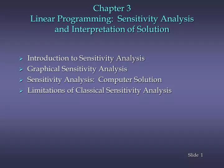
Chapter 3 Linear Programming: Sensitivity Analysis and Interpretation of Solution. Introduction to Sensitivity Analysis Graphical Sensitivity Analysis Sensitivity Analysis: Computer Solution Limitations of Classical Sensitivity Analysis. Introduction to Sensitivity Analysis.

E N D
Chapter 3 Linear Programming: Sensitivity Analysis and Interpretation of Solution • Introduction to Sensitivity Analysis • Graphical Sensitivity Analysis • Sensitivity Analysis: Computer Solution • Limitations of Classical Sensitivity Analysis
Introduction to Sensitivity Analysis In the previous chapter we discussed: • objective function value • values of the decision variables • slack/surplus In this chapter we will discuss: • changes in the coefficients of the objective function • changes in the right-hand side value of a constraint • reduced costs
Introduction to Sensitivity Analysis Sensitivity analysis (or post-optimality analysis) is used to determine how the optimal solution is affected by changes, within specified ranges, in: • the objective function coefficients • the right-hand side (RHS) values Sensitivity analysis is important to a manager who must operate in a dynamic environment with imprecise estimates of the coefficients. Sensitivity analysis allows a manager to ask certain what-if questions about the problem.
Graphical Sensitivity Analysis For LP problems with two decision variables, graphical solution methods can be used to perform sensitivity analysis on • the objective function coefficients, and • the right-hand-side values for the constraints. XYZ, Inc. LP Formulation Max Z = 5x1 + 7x2 s.t. x1< 6 (1) 2x1 + 3x2< 19 (2) x1 + x2< 8 (3) x1, x2> 0
Example 1 Graphical Solution x2 x1 + x2< 8 (3) 8 7 6 5 4 3 2 1 Max 5x1 + 7x2 x1< 6 (1) Optimal Solution: x1 = 5, x2 = 3, Z= 46 2x1 + 3x2< 19 (2) x1 1 2 3 4 5 6 7 8 9 10
Objective Function Coefficients The range of optimality for each coefficient provides the range of values over which the values of decision variables will remain optimal (i.e., the same). Note that the objective function value will change if the coefficient/s of the decision variable/s is/are changed. E.g., Suppose now the new objective function is Maximize Z = 6x1 + 7x2. What is the new optimal solution (i.e., x1, x2, and Z)?
Example 1 Changing Slope of Objective Function x2 Coincides with x1 + x2< 8 (3) constraint line 8 7 6 5 4 3 2 1 Objective function line for 5x1 + 7x2 5 Coincides with 2x1 + 3x2< 19 (2) constraint line Feasible Region 4 3 1 2 x1 1 2 3 4 5 6 7 8 9 10
Range of Optimality Graphically, the limits of a range of optimality are found by changing the slope of the objective function line within the limits of the slopes of the binding constraint lines. Slope of an objective function line, Max c1x1 + c2x2, is -c1/c2, and the slope of a constraint, a1x1 + a2x2 = b, is -a1/a2. Example: XYZ, Corp. Objective function: 5x1 + 7x2 Slope of objective function = - 5/7
Example 1 Range of Optimality for c1 The slope of the objective function line is -c1/c2. The slope of the first binding constraint, x1 + x2 = 8, is -1 and the slope of the second binding constraint, 2x1 + 3x2 = 19, is -2/3. Find the range of values for c1 (with c2 staying 7) such that the objective function line slope lies between that of the two binding constraints: -1 < -c1/7 < -2/3 Multiplying through by -7 (and reversing the inequalities): 14/3 <c1< 7
Example 1 Range of Optimality for c1 Would a change in c1 from 5 to 7 (with c2 unchanged) cause a change in the optimal values of the decision variables (i.e., x1 and x2)? The answer is ‘no’ because when c1 = 7, the condition 14/3 <c1< 7 is satisfied. What about the optimal value of the objective function, Z? Would a change in c1 from 5 to 8 (with c2 unchanged) cause a change in the optimal x1, x2 and Z? Why?
Example 1 Range of Optimality for c2 Find the range of values for c2 ( with c1 staying 5) such that the objective function line slope lies between that of the two binding constraints: -1 < -5/c2< -2/3 Multiplying by -1: 1 > 5/c2> 2/3 Inverting, 1 <c2/5 < 3/2 Multiplying by 5: 5 <c2< 15/2
Example 1 Range of Optimality for c2 Would a change in c2 from 7 to 6 (with c1 unchanged) cause a change in the optimal values of the decision variables? The answer is ‘no’ because when c2 = 6, the condition 5 <c2< 15/2 is satisfied. Would a change in c2 from 7 to 8 (with c1 unchanged) cause a change in the optimal decision variables and optimal objective function value? Why?
Important Notes • The range of optimality for objective function coefficients is only applicable for changes made to one coefficient at a time. • All other coefficients are assumed to be fixed. • If two or more coefficients are changed simultaneously, further analysis is usually necessary. • However, when solving two-variable problems graphically, the analysis is fairly easy. • Simply compute the slope of the objective function (-Cx1/Cx2 ) for the new coefficient values. • If this ratio is > the lower limit on the slope of the objective function and < the upper limit, then the changes made will not cause a change in the optimal solution.
Example 1 Simultaneous Changes in c1 and c2 Would simultaneously changing c1 from 5 to 7 and changing c2 from 7 to 6 cause a change in the optimal solution? (Recall that these changes individually did not cause the optimal solution to change.) Recall that the objective function line slope must lie between that of the two binding constraints: -1 < -c1/c2< -2/3 The answer is ‘yes’ the optimal solution (i.e., x1, x2 and Z) changes because -7/6 does not satisfy the above condition.
Right-Hand Sides • Let us consider how a change in the right-hand side for a constraint might affect the feasible region and perhaps cause a change in the optimal solution. • The change in the value of the optimal solution per unit increase in the right-hand side is called the dual value. • The range of feasibility is the range over which the dual value is applicable. • As the RHS increases sufficiently, other constraints will become binding and limit the change in the value of the objective function.
Dual Value • Graphically, a dual value is determined by adding +1 to the right hand side value in question and then resolving for the optimal solution in terms of the same two binding constraints. • The dual value is equal to the difference in the values of the objective functions between the new and original problems. • Note that all the optimal values (i.e., all the decision variables and objective function value) will change when you change the right hand side value/s of the binding constraint/s. • The dual value for a nonbinding constraint is 0.
Example 1 Dual Values Constraint 1: Since x1< 6 is not a binding constraint, its dual price is 0. Constraint 2: Change the RHS value of the second constraint to 20 and resolve for the optimal point determined by the last two constraints: 2x1 + 3x2 = 20 and x1 + x2 = 8. The solution is x1 = 4, x2 = 4, z = 48. Hence, the dual price = znew - zold = 48 - 46 = 2. Constraint 3: Change the RHS value of the third constraint to 9 and resolve for the optimal point determined by the last two constraints: 2x1 + 3x2 = 19 and x1 + x2 = 9. The solution is: x1 = 8, x2 = 1, z = 47. The dual price is znew - zold = 47 - 46 = 1.
Range of Feasibility • Note that when the right hand side value of a binding constraint is changed allthe values (i.e., x1, x2 and Z) of the optimal solution will also change. • Graphically, the range of feasibility is determined by finding the values of a right hand side coefficient such that the same two lines that determined the original optimal solution continue to determine the optimal solution for the problem. • The range of feasibility for a change in the right hand side value is the range of values for this coefficient in which the original dual value remains constant.
Sensitivity Analysis: Computer Solution Software packages, such as QM for Windows, provide the following LP information: Information about the objective function: • its optimal value • coefficient ranges (ranges of optimality) Information about the decision variables: • their optimal values • their reduced costs Information about the constraints: • the amount of slack or surplus • the dual prices • right-hand side ranges (ranges of feasibility)
Reduced Cost • The reduced cost for a decision variable whose value is 0 in the optimal solution is: the amount the variable's objective function coefficient would have to improve (increase for maximization problems, decrease for minimization problems) before this variable could assume a positive value. • The reduced cost for a decision variable whose value is > 0 in the optimal solution is 0.
Important Notes onthe Interpretation of Dual Values • Resource cost is sunk (i.e., fixed) • The dual value is the maximum amount you should be willing to pay for one additional unit of the resource. • Sunk resource costs are not reflected in the objective function coefficients. • Resource cost is relevant (i.e., variable) • The dual value is the maximum premium over the variable cost that you should be willing to pay for one additional unit of the resource. • Relevant costs are reflected in the objective function coefficients.
Computer Solutions: XYZ. Inc. For MAN 321, we will use QM for Windows Spreadsheet Showing Problem Data
Computer Solutions: XYZ. Inc. Spreadsheet Showing Solution
Computer Solutions: XYZ. Inc. Spreadsheet Showing Ranging Note: Slacks/Surplus and Reduced Costs