Download
1 / 30
300 likes | 306 Vues
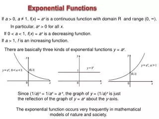
10.5 Using Exponential Functions to Model Data. Exponential model, exponentially related, approximately exponentially related. Definition.

E N D
Exponential model, exponentially related, approximately exponentially related Definition If no exponential curve contains all of the data points, but an exponential curve comes close to all of the data points (and perhaps contains some of them), then we say the variables are approximately exponentially related.
Example: Modeling with an Exponential Function Suppose that a peach has 3 million bacteria on it at noon on Monday and that one bacterium divides into two bacteria every hour, on average.
Example: Modeling with an Exponential Function Let B = f(t) be the number of bacteria (in millions) on the peach at t hours after noon on Monday. 1. Find an equation of f. 2. Predict the number of bacteria on the peach at noon on Tuesday.
Solution 1. We complete a table of value of f based on the assumption that one bacterium divides into two bacteria every hour.
Solution 1. As the value of t increases by 1, the value of B changes by greater and greater amounts, so it would not be appropriate to model the data by using a linear function. Note, though, that as the value of t increases by 1, the value of B is multiplied by 2, so we can model the situation by using an exponential model of the form f(t) = a(2)t. The B-intercept is (0, 3), so f(t) = 3(2)t.
Solution 1. Use a graphing calculator table and graph to verify our work.
Solution 2. Use t = 24 to represent noon on Tuesday. Substitute 24 for t in our equation of f: f(24) = 3(2)24 = 50,331,648 According to the model, there would be 50,331,648 million bacteria. To omit writing “million,” we must add six zeroes to 50,331,648 – that is 50,331,648,000,000. There would be able 50 trillion bacteria at noon on Tuesday.
Exponential Model y = abt If y = abt is an exponential model where y is a quantity at time t, then the coefficient a is the value of that quantity present at time t = 0. For example, the bacteria model f(t) = 3(2)t has coefficient 3, which represents the 3 million bacteria that were present at time t = 0.
Example: Modeling with an Exponential Function A person invests $5000 in an account that earns 6% interest compounded annually. 1. Let V = f(t) be the value (in dollars) of the account at t years after the money is invested. Find an equation of f. 2. What will be the value after 10 years?
Solution 1. Each year, the investment value is equal to the previous year’s value (100% of it) plus 6% of the previous year’s value. So, the value is equal to 106% of the previous year’s value.
Solution 1. As the value of t increases by 1, the value of V is multiplied by 1.06. So, f is the exponential function f(t) = a(1.06)t. Since the value of the account at the start is $5000, we have a = 5000. So, f(t) = 5000(1.06)t.
Solution 2. To find the value in 10 years, substitute 10 for t: f(10) = 5000(1.06)10 ≈ 8954.24 The value will be $8954.24 in 10 years.
Half-life Definition If a quantity decays exponentially, the half-life is the amount of time it takes for that quantity to be reduced to half.
Example: Modeling with an Exponential Function The world’s worse nuclear accident occurred in Chernobyl, Ukraine, on April 26, 1986. Immediately afterward, 28 people died from acute radiation sickness. So far, about 25,000 people have died from the accident, mostly due to the release of the radioactive element cesium-137 (Source: Medicine Worldwide).
Example: Modeling with an Exponential Function Cesium-137 has a half-life of 30 years. Let P = f(t) be the percent of the cesium-137 that remains at t years since 1986. 1. Find an equation of f. 2. Describe the meaning of the base of f. 3. What percent of the cesium-137 will remain in 2015?
Solution 1. We discuss two methods of finding an equation of f. Method 1 The table shows the values of P at various years t. The data can be modeled well with an exponential function. So,
Solution 1. We can use a graphing calculator table and graph to verify our equation. Write this equation in the form f(t) = abt: Since we can write P = f(t) = 100(0.977)t
Solution 1. Method 2 Instead of recognizing a pattern from the table, we can find an equation of f by using the first two points on the table, (0,100) and (30, 50). Since the P-intercept is (0, 100), we have P = f(t) = 100bt
Solution 1. To find b, we substitute the coordinates of (30, 50) into the equation: So, an equation of f is f(t) = 100(0.977)t, the same equation we found using Method 1.
Solution 2. The base of f is 0.977.Each year, 97.7% of the previous year’s cesium-137 is present. In other words, the cesium-137 decays by 2.3% each year. 3. Since 2015 – 1986 = 29, substitute 29 for t: f(29) = 100(0.977)29 ≈ 50.9263 In 2015, about 50.9% of the cesium-137 will remain.
Meaning of the Base of an Exponential Model • If f(t) = abt, where a > 0, models a quantity at time t, then the percent rate of change is constant. In particular, • If b > 1, then the quantity grows exponentially at a rate of b – 1 percent (in decimal form) per unit of time. • If 0 < b < 1, then the quantity decays exponentially at a rate of 1 – b percent (in decimal form) per unit of time.
Example: Modeling with an Exponential Function The number of severe near collisions on airplane runways has decayed approximately exponentially from 67 in 2000 to 16 in 2010 (Source: Federal Aviation Administration). Predict the number of severe near collisions in 2015.
Solution Let n be the number of severe near collisions on airplane runways in the year that is t years since 2000. Known values of t and n are shown in the table below.
Solution Because the variables t and n are approximately exponentially related, we want an equation in the form n = abt. The n-intercept is (0, 67). So, the equation is of the form n = 67bt
Solution To find b, substitute (10, 16) into the equation and solve for b:
Solution Substitute 0.867 for b in the equation n = 67bt: n = 67(0.867)t Finally, to predict the number of severe near collisions in 2015, substitute 2015 – 2000 = 15 for t in the equation and solve for n: n = 67(0.867)15 ≈ 7.88
Solution The model predicts that there will be about 8 severe near collisions in 2015. We use a graphing calculator table to check that each of the three ordered pairs (0, 67), (10, 16), and (15, 7.88) approximately satisfies the equation n = 67(0.867)t.
Four-Step Modeling Process To find a model and then make estimates and predictions, 1. Create a scattergram of the data. Decide whether a line, a parabola, an exponential curve, or none of these comes close to the points. 2. Find the equation of your model.
Four-Step Modeling Process 3. Verify your equation has a graph that comes close to the points in the scattergram. If it doesn’t, check for calculation errors or use different points to find the equation. An alternative is to reconsider your choice of model in step 1. 4. Use your equation of the model to draw conclusions, make estimates, and/or make predictions.