Download

1 / 39
390 likes | 508 Vues
FSM State Assignment for Area, Power and Testability using Modern Optimization Techniques. Mohammed Mansoor Ali Computer Engineering Department. Outline. Introduction Finite State Machines (FSMs) FSM State Assignment (Encoding) FSM Encoding for Area FSM Encoding for Power

E N D
FSM State Assignment for Area, Power and Testability using Modern Optimization Techniques Mohammed Mansoor Ali Computer Engineering Department
Outline • Introduction • Finite State Machines (FSMs) • FSM State Assignment (Encoding) • FSM Encoding for Area • FSM Encoding for Power • FSM Encoding for Testability • Modern Iterative Heuristics • Simulated Evolution (SimE) • Conclusions
Introduction • Complexity of VLSI circuits is constantly increasing. • Design partitioning and abstraction are commonly employed to tackle the complexity. • CAD tools are employed at different levels of design hierarchy to ease the flow. • The performance of CAD tools in turn depends on how well the problem can be modeled or in other words how efficient are cost-metrics.
Finite State Machines • Digital systems are composed of a data-path and a controller • The controller utilizes present state values to decide the sequence of operations to be performed next in the data-path. • A finite number of storage elements are employed to store finite number of present state values. Thus another name of such a controller is Finite State Machine (FSM). • FSM synthesis have been a central problem in the design of digital systems.
Finite State Machines • An FSM can be thought of as purely a combinational circuit whose (some) previous outputs are utilized in evaluating (some) current outputs. • The previous outputs are stored in a binary coded form in some storage elements. Such codes are also known as states of the state machine. • Thus, FSM is a combination of a combinational circuit and some storage elements. • The combinational component is responsible for producing outputs depending on state values and/or inputs. • Thus, the complexity of combinational circuit is thus a function of its outputs, i.e. state codes as well as external outputs of the machine.
FSM State Assignment • One of the main problems in the synthesis of sequential machines • Plays a major role in the complexity of the FSM’s combinational circuit (and hence the area). • Also, power and testability of an FSM are functions of state assignment
FSM State Assignment • FSM State assignment is an NP hard problem • Huge number of possible encoding combinations where nb is number of encoding bits used and s are number of states For e.g. a 10 state using 4 bits to encode 29.05 x10^9 combinations
FSM Encoding for Area • Area is a function of • Number of storage bits • Type of flip-flop employed • Encoding of the states • Minimum number of state variables needed for state assignment • Use of D-type flip-flops is most prevalent in VLSI circuits today. • Logic minimization tools aim to optimize the combinational logic of an FSM. • A good encoding can help the logic minimizer to achieve a better realization in terms of logic cost. • Logic minimization target two-level and multi-level circuit implementations independently.
FSM Encoding for Area • 2-level logic minimization utilizes attributes • Code-covering • Implicant merging • Disjunctive coding • Multi-level minimization utilizes attributes like factorization and decomposition for common cube extraction and literal savings. • Carefully chosen state code helps logic minimizers to achieve better realization of the sequential circuit. • Such attributes and their inter-effects are difficult to predict while doing state encoding.
Two Level Implementation • Realize a logic function as a sum of product terms. • The circuit complexity is related to • Number of inputs • Number of outputs • Number of product terms • Number of variables utilized in a product term i.e. the number of literals. • Complexity can be reduced by using mechanisms such as implicant merging, code covering and disjunctive coding.
Implicant Merging • Assign adjacent codes to states that produce either same next-state or output or both at similar input conditions. • Yields bigger cubes while doing Karnaugh minimization, and resulting in a simpler final expression. • Implicant merging requires adjacency constraints to be met by the state assignment algorithm.
Code Covering • Involves a code word of a state covering code word of some other state (s) • Covering constraints produce covering code words.
Disjunctive Coding • Require that disjunction of state codes is equal to some other state code.
Problems • Major difficulty for 2-level realization of an FSM is the simultaneous consideration of all the types of constraints. • Not possible to satisfy all the coding conditions with a code using the minimum number of bits r0. • By increasing the number of code bits to r > r0, more coding constraints can be satisfied. • Increase in the number of storage elements and state signals to be generated has to be justified • No exact predictions are possible, as to how the satisfaction of coding conditions affects the complexity of the resulting combinational logic, • The application of coding constraint and finding out their effect would be excessively costly as it would require a huge number of logic minimizations
Multi-Level Minimization • Provides more degree of freedom in optimizing combinational network and satisfying coding constraints. • Flexibility provided due to operations such as common sub-expression extraction and factorization. • Increase in difficulty of modeling and optimizing the multilevel network themselves. • Complexity measure for multilevel circuits is the encoding length and the number of literals in the optimized logic network.
Jedi Area Measure • Encoding affinity cost is modeled as a function of how many times a pair of states are represented in next state and output functions. Po k;i is number of times output k is represented in output i, Po k;i is number of times state k is represented in state i, mo is the number of outputs, ns is the number of states, nE is the number of encoding bits.
Mustang Area Measure • Mustang observed that two states for which the frequencies of same next state are 50 and 2 are less strongly connected than the states which have frequencies 26 and 26. • Thus approximated + with *
Expand Area Measure • Expand function used in ESPRESSO tool can also be utilized in multi-level area measure. • Goal of Expand function is to increase the size of each implicant of a given cover F so that implicants of smaller size can be covered and deleted. • Maximally expanded implicants are primes of the function
FSM Encoding for Power • Power is consumed due to toggling within the combinational circuit as well as on the state lines. • Switching can be reduced • By minimizing the area • By minimizing the number of inputs to the combinational component • By minimizing the average switching on the inputs feeding the combinational network. • Lesser Hamming Distance between frequently reduces the average switching • Problem translated to finding states that have frequent transitions in between.
Power Estimation • Static vs. Probabilistic approach • The statistical approaches work by • Simulating the state machine using the user provided input vectors • Determining the state probabilities based on it. • Fast and accurate if a short representative sequence for an FSM can be determined. • However, determining such a sequence is an open research problem. • Probabilistic approaches on the other hand try to • Correlate the various probabilities in order to calculate state probabilities if the FSM is simulated for infinite amount of time. • Requires a set of iterative equations known as Chapman- Kolmogorov equations.
Power Estimation • State Transition Graph (STG) denoted by G(V, E) • Vertex Siє V represents a state of the FSM • Edge ei,jє E represents a transition from state Sito Sj. • PSidenote the state probability • Probability of finding the state machine in Si at any given time • pijdenotes the state transition probability • Probability of the machine making a transition from state Sito state Sj
Power Estimation • Total State Transition Probability for a transition from a state Si to state Sj can be calculated as: • Using Markov Chains and Chapman-Kolmogorov equations • The sum of total state transition probabilities in between two states indicates the amount of switching in between them. • Can be treated as a weight between the two states attributed on a single edge connecting them.
Power Estimation • The STG is now a weighted graph. • The weight on an edge indicates the relative proximity in the state assignment of the two connected states on that edge. • Overall switching can be minimized by assigning shorter distance codes to states connected with higher weights, • Minimum Weighted Hamming Distance (MWHD).
FSM Encoding for Testability • Testability attributed to how efficiently a circuit lets the excitation and observation of faults on application of test vectors. • More excitable and observable if it has a high switching probability. • Test generation for combinational circuit is itself a hard problem. • Sequential circuits employ memory elements • Require an added domain of time for their testing. • Complexity of acyclic sequential circuit • comparable to the complexity of a combinational circuit (d*2i) • Complexity increases exponentially • with the number and length of cycles (loops)
Testability • Involves • Generation and application of test sets at primary inputs • Excite its various faults • Observing them at the outputs. • Can either be manually generated or using automatic CAD tools. • Automatic test generation tools are efficient in terms of cost and effectiveness • Use both random and deterministic techniques to build the test set. • Deterministic test set • Takes into account the behavior and structure of the circuit under test to build its test set. • Yield higher fault coverage but computationally expensive. • The complexity and type of a circuit, determines how efficiently automatic test pattern generator performs.
Testability • The worst case size of the search space is bounded by 2i, where i is equal to the number of inputs. • However, techniques have been developed to reduce this large search space by an intelligent search of the primary input combinations. • These techniques include D-algorithm, PODEM, and FAN. • A sequential circuit can be classified as cyclic or acyclic. • Sequential depth refers to the number of sequential elements from primary input to the primary output.
Cost Function for Testability • Calculate depth of all loops in the synthesized circuit • Estimate uninitializability of a circuit resulting from an assignment • Try to favor initializable implementations. • The initialized flip-flops can later on be used for initializing the rest of the sequential elements.
Cost Function for Testability • Logic-High Initialization: A flip-flop can be initialized to logic-high if there exists an implicant in its cover that only depends on inputs. • Logic-Low Initialization: A flip-flop can be initialized to logic-low if there exists an implicant in its complement cover that only depends on inputs
Iterative Heuristics • Combinational optimization algorithms: • Exact Algorithms • dynamic programming, branch and-bound, backtracking, etc • Approximation Algorithms (Heuristic Methods) • Many of the significant optimization problems NP-Hard. • Genetic Algorithms, Tabu Search, Simulated Evolution, etc.
Simulated Evolution • SimE is a general iterative heuristic proposed by Ralph Kling • Combines iterative improvement and constructive perturbation • Saves itself from getting trapped in local minima by following a stochastic perturbation approach. • Selection of which components of a solution to change is done according to a stochastic rule. • Already well located components have a high probability to remain where they are. • The probabilistic feature gives SimE hill-climbing property.
Simulated Evolution • It is general in the sense that it can be tailored to solve most known combinatorial optimization problems • It has the capability of escaping local minima • It is blind, i.e., it does not know the optimal solution and has to be told when to stop.
Evaluation • Consists of evaluating the goodness of each individual i of the population P. • Goodness measure must be a single number expressible in the range [0; 1]. • Goodness can be defined as follows: • Oiis an estimate of the optimal cost of individual i, and Ciis the actual cost of i in its current location. • Oiis calculated only once at the beginning of simulation.
Evaluation • Desired Adjacency Graph (DAG): • Armstrong defined adjacency as a combination of fan-out and fan-in approaches. • The higher the DAG value, the more desirable the states should be closer • Another goodness measure: • Function of DAG and Hamming Distance • What else???
Selection • Takes as input • population P • Estimated goodness of each individual • Partitions P into two disjoint sets • A selection set Ps • A set Pr of the remaining members of the population . • Each member of the population is considered separately from all other individuals. • The decision whether to assign individual i to the set Psor set Pris based solely on its goodness gi.
Allocation • Has most impact on the quality of solution. • Takes as input the two sets Ps and Pr • Generates a new population P0 which contains all the members of the previous population P, with the elements of Ps mutated. • The choice of a suitable Allocation function is problem specific. • Usually, a number of trial-mutations are performed and rated with respect to their goodnesses. • Based on the resulting goodnesses, a final configuration of the population P0 is decided. • The goal of Allocation is to favor improvements over the previous generation, without being too greedy.
Conclusions • FSM encoding have been a central problem in the design of digital systems • Plays a major role in the complexity of the FSMs combinational circuit • Power and testability of an FSM are functions of state assignment • Various cost measures have been proposed. • From the results reported in the literature SimE algorithm is a sound and robust randomized search heuristic. • It is guaranteed to converge to the optimal solution if given enough time.
Q & A Thank You