Download
1 / 39
400 likes | 565 Vues
Magnetic vector potential. For an electrostatic field We cannot therefore represent B by e.g. the gradient of a scalar since Magnetostatic field, try B is unchanged by. 5). Magnetic Phenomena. Electric polarisation ( P ) - electric dipole moment per unit vol.

E N D
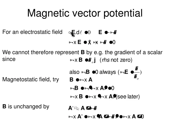
Magnetic vector potential For an electrostatic field We cannot therefore represent B by e.g. the gradient of a scalar since Magnetostatic field, try B is unchanged by
5). Magnetic Phenomena Electric polarisation (P) - electric dipole moment per unit vol. Magnetic polarisation (M) - magnetic dipole moment per unit vol. Mmagnetisation Am-1 c.f. P polarisation Cm-2 Element magnetic dipole moment m When all moments have same magnitude & directionM=Nm N number density of magnetic moments Dielectric polarisation described in terms of surface (uniform) or volume (non-uniform) bound charge densities By analogy, expect description in terms of surface (uniform) or volume (non-uniform) magnetisation current densities
Definitions • Electric polarisation P(r) Magnetic polarisation M(r) p electric dipole moment of m magnetic dipole moment of localised charge distribution localised current distribution
a f Magnetic moment of current loop For a planar current loop m = I A z A m2 z unit vector perpendicular to plane
v4 r5 v5 v1 r4 O r1 r3 r2 v3 v2 Magnetic moment and angular momentum • Magnetic moment of a group of electrons m • Charge –e mass me
F r q T r m L q I B F Torque on magnetic moment p/2-q F L/2 dq L/2 F
-e a I Origin of permanent magnetic dipole moment non-zero net angular momentum of electrons Includes both orbit and spin Derive general expression via circular orbit of one electron radius: a charge: -e mass: me speed: v ang. freq: ang. momentum: L dipole moment:m Similar expression applies for spin.
L -e m Origin of permanent magnetic dipole moment Consider directions: m and L have opposite sense In general an atom has total magnetic dipole moment: ℓquantised in units of h-bar, introduce Bohr magneton
B -e +Ze -e Diamagnetic susceptibility (mr < 1) Characterised by mr < 1 In previous analysis of permanent magnetic dipole moment, m = 0 when net L = 0: now look for induced dipole moment Applied magnetic field causes small change in electron orbit, leading to induced L, hence induced m Consider force balance equation when B = 0 (mass) x (accel) = (electric force) If B perp to orbit (up), extra inwards Lorentz force: Approx: radius unchanged, ang. freq increased from wo to w
Larmor frequency (wL) balance equation when B ≠ 0 (mass) x (accel) = (electric force) + (extra force) wL is known as the Larmor frequency
m a -e v -e v -e v x B -e v x B m Classical model for diamagnetism • Pair of electrons in a pz orbital B • = wo - wL |ℓ| = -mewLa2 m = -e/2me ℓ • = wo + wL |ℓ| = +mewLa2 m = -e/2me ℓ Electron pair acquires a net angular momentum/magnetic moment
B -e m Induced dipole moment • Increase in ang freq increase in ang mom (ℓ) • increase in magnetic dipole moment: Include all Z electrons to get effective total induced magnetic dipole moment with sense opposite to that of B
Critical comments on last expression Although expression is correct, its derivation is not formally correct (no QM!) It implies that ℓis linear in B, whereas QM requires that ℓ is quantised in units of h-bar Fortunately, full QM treatment gives same answer, to which must be added any paramagnetic-contribution everything is diamagnetic to some extent
Bdip Bappl Bappl Paramagnetic media (mr > 1) analogous to polar dielectric alignment of permanent magnetic dipole moment in applied magnetic field B An aligned electric dipole opposes the applied electric field; But here the dipole field adds to the applied field! Other than that, it is completely analogous in thermal effect of disorder etc., hence use Langevin analysis again
Langevin analysis of paramagnetism As with polar dielectric media, the field B in the expressions should be the local field Bloc but generally find Bloc ≈ B
Uniform magnetisation Electric polarisation Magnetic polarisation Magnetisation is a current per unit length For uniform magnetisation, all current localised on surface of magnetised body (c.f. induced charge in uniform polarisation) I z y x
m M Surface Magnetisation Current Density Symbol: aM ; a vector current density but note units: Am-1 Consider a cylinder of radius r and uniform magnetisation M where M is parallel to cylinder axis Since M arises from individualm, (which in turn arise in current loops) draw these loops on the end face Current loops cancel in volume, leaving net surface current.
aM M Surface Magnetisation Current Density magnitude aM = M but for a vector must also determine its direction aM is perpendicular to both M and the surface normal Normally, current density is “current per unit area” in this case it is “current per unit length”, length along the Cylinder - analogous to current in a solenoid.
I L Solenoid with magnetic core Recap, vacuum solenoid: With magnetic core (red), Ampere’s Law encloses two types of current, “conduction current” in the coils and“magnetisation current” on the surface of material: r > 1: aM and I in same direction (paramagnetic) r < 1: aM and I in opposite directions (diamagnetic) Substitute for aM : (see later)
z I1-I2 I2-I3 My I1 I2 I3 x Non-uniform magnetisation A rectangular slab of material in which M is directed along y-axis only but increases in magnitude along the x-axis only As individual loop currents increase from left to right, there is a net “mag current” along the z-axis, implying a “mag current density” which we will call
dx dx Neighbouring elemental boxes Consider 3 identical element boxes, centres separated by dx If the circulating current on the central box is Then on the left and right boxes, respectively, it is
Upward and circulating currents The “mag current” is the difference in neighbouring circulating currents, where the half takes care of the fact that each box is used twice! This simplifies to
My -Mx I1-I2 I2-I3 z z y x I1 I2 I3 x Non-uniform magnetisation A rectangular slab of material in which M is directed along -x-axis only but increases in magnitude along the y-axis only Total magnetisation current || z Similar analysis for x, y components yields
Magnetic Field Intensity H Recall Ampere’s Law Recognise two types of current, free and bound
Ib If If L L Ampere’s Law for H Often more useful to apply Ampere’s Law for H than for B Bound current in magnetic moments of atoms Free current in conduction currents in external circuits or metallic magnetic media
Magnetic Susceptibility B • Two definitions of magnetic susceptibility • First M = BB/mo is analogous to P = eoEE • B, field due to all currents, E, field due to all charges • B r • Au -3.6.10-5 0.99996 • Quartz -6.2.10-5 0.99994 • O2 STP +1.9.10-6 1.000002 • In this definition the diamagnetic susceptibility is negative and • the relative permeability is less than unity c.f. D = ereoE
1.5 B(T) 0 -500 +500 -1.5 H Am-1 Magnetic Susceptibility M • Second definition not analogous to P = eo E E • When is much less than unity (all except ferromagnets) the • two definitions are roughly equivalent Para-, diamagnets Ferromagnet m ~ 150-5000 for Fe Hysteresis and energy dissipation
1 2 B1 q1 B2 q1 dℓ1 H1 1 B A C Ienclfree q2 2 q2 H2 dℓ2 S Boundary conditions on B, H For LIH magnetic media B = mmoH (diamagnets, paramagnets, not ferromagnets for which B = B(H))
E B dℓ S Faraday’s Law
B(r) I Faraday’s Law To establish steady current, cell must do work against Ohmic losses and to create magnetic field
j da dℓ Energy density in magnetic fields
Time variation Combining electrostatics and magnetostatics: (1) .E = r/eo wherer=rf+ rb (2) .B = 0 “no magnetic monopoles” (3) x E = 0 “conservative” (4) x B = moj where j= jf + jM Under time-variation: (1) and (2) are unchanged, (3) becomes Faraday’s Law (4) acquires an extra term, plus 3rd component of j
B dS dℓ Faraday’s Law of Induction emfx induced in a circuit equals the rate of change of magnetic flux through the circuit
Problem! Displacement current Ampere’s Law Continuity equation Steady current implies constant charge density so Ampere’s law consistent with the Continuity equation for steady currents Ampere’s law inconsistent with the continuity equation (conservation of charge) when charge density time dependent
Extending Ampere’s Law add term to LHS such that taking Div makes LHS also identically equal to zero: The extra term is in the bracket extended Ampere’s Law
k M= sin(ay) k j i jM= curl M = a cos(ay) i Types of current j Total current • Polarisation current density from oscillation of charges in • electric dipoles • Magnetisation current density variation in magnitude of • magnetic dipoles in space/time