Download
1 / 19
190 likes | 311 Vues
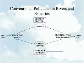
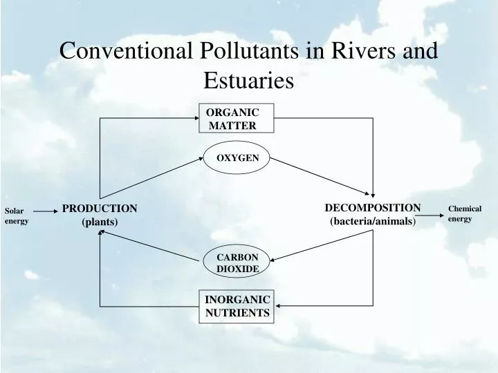
Conventional Pollutants in Rivers and Estuaries. ORGANIC MATTER. OXYGEN. DECOMPOSITION (bacteria/animals ). PRODUCTION (plants). Chemical energy. Solar energy. CARBON DIOXIDE. INORGANIC NUTRIENTS. Principle of Superposition. Mass balance for DO deficit In terms of L and N.

E N D
Conventional Pollutants in Rivers and Estuaries ORGANIC MATTER OXYGEN DECOMPOSITION (bacteria/animals) PRODUCTION (plants) Chemical energy Solar energy CARBON DIOXIDE INORGANIC NUTRIENTS
Principle of Superposition • Mass balance for DO deficit • In terms of L and N
PHOTOSYNTHESIS CHARACTERISTICS • Dissolved oxygen deficit mass balance
function ee=errordef(x) ka=x(1); Pm=x(2); Dm=x(3); dox=[…] tt=[…] n=10; f=13./24; bn=1:2; for i=1:10 bn(i)=cos(i*pi*f)*4*pi/f/((pi/f)^2-(2*pi)^2*i*i); end d=1:24; Tp=1.; for t=1:24 d(t)=Dm; for i=1:10 d(t)=d(t)-Pm*bn(i)/(ka^2+(2*pi*i/Tp)^2)^0.5* ... cos(2*pi*i/Tp*(t/24.-f*Tp/2.)-atan(2*pi*i/ka/Tp)); end end ta=tt+273.15; os=ta; for i=1:24 os(i)=-139.34411+1.575701e5/ta(i)- … 6.642308e7/ta(i)^2+1.2438e10/ta(i)^3- ... 8.621949e11/ta(i)^4; end os=exp(os); d=os-d; ee=norm(dox-d);
DYNAMIC APPROACH • Routing water (St. Venant equations) • Continuity equation • Momentum equation (Local acceleration + Convective acceleration+pressure + gravity + friction = 0 Kinematic wave Diffusion wave Dynamic wave
KINEMATIC ROUTING • Geometric slope = Friction slope • Manning’s equation • Express cross section area as a function of flow
KINEMATIC ROUTING (ctd) • Express the continuity equation exclusively as a function of Q • Discretize continuity equation and solve it numerically k+1 t k 1 2 3 4 5 n n-1 n x
KINEMATIC ROUTING (ctd) • Discretize continuity equation and solve it numerically • Example • Q=2.5m3s-1; S0=0.004 • B=15m; n0=0.07 • Qe=2.5+2.5sin(wt); w=2pi(0.5d)-1
S0=0.004; B=15; n0=0.07; n=80; Q=zeros(2,n)+2.5; dx=1000.; %meters dt=700.; %seconds alpha=(n0*B^(2./3.)/sqrt(S0))^(3./5.) beta=3./5.; for it=1:150 if it*dt/24/3600 < 0.25 Q(2,1)=2.5+2.5* … sin(2.*pi*it*dt/(0.5*24*3600)); else Q(2,1)=2.5; end for i=2:n Q(2,i)=(dt/dx*Q(2,i-1)* … ((Q(1,i)+Q(2,i-1))/2.)^(1-beta)... +alpha*beta*Q(1,i))/… (dt/dx*((Q(1,i)+Q(2,i-1))/2.)^(1-beta)... +alpha*beta); end Q(1,:)=Q(2,:); if floor(it/40)*40==it x=1:n; plot(x,Q(1,:)); hold on end end
ROUTING POLLUTANTS • Mass conservation • Discretized mass balance equation k+1 t k 1 2 3 4 5 n n-1 n x
ROUTING POLLUTANTS (ctd) • Alternate formulation • Example • u = 1 ms-1 • x = 1000 m • t = 500 m
ROUTING POLLUTANTSNumerical Example u=1.; %m/s dx=1000; %m dt=500; %s n=100; x=1:100; y=x-20; c0=exp(-0.015*y.*y); c1=c0; plot(x,c0); hold on for it=1:120 for i=2:n-1 c1(i)=c0(i)+u*dt/dx* … (c0(i-1)-c0(i)); end c0=c1; if fix(it/40)*40==it plot(x,c0); end end xlabel('x (km)'); ylabel('C mgL^{-1}');
ROUTING POLLUTANTS (ctd) • Second order (both time and space) formulation • Stability condition
ROUTING POLLUTANTS (ctd) • Numerical oscillations
OXYGEN BALANCE GENERAL NUMERICAL APPROACH 1 • Do spatial discretization • Route the water for each reach • Apply water continuity at junctions • Q8+Q15=Q16 • Route the pollutants for each reach • Apply pollutant continuity junctions • Solve the production/decomposition for each grid point Reach 1 2 3 9 4 10 11 5 12 6 13 14 7 Reach 2 15 8 16 17 18 19 Reach 3 20 21 22
Sensitivity Analysis • First order analysis • y=f(x) • y0=f(x0)
Sensitivity Analysis • Monte Carlo Analysis • 1. Generate dx0 = N(0,x) • 2. Determine y=f(x0+dx0) • 3. Save Y={Y | y} • 4. i=i+1 • 5. If i < imax go to 1 • 6. Analyze statistically Y
xspan=0:100; %parameter definition Lr=zeros(100,101); Dr=zeros(100,101); global ka kd U U=16.4; y0=[10 0]'; %initial concentrations are given in mg/L for i=1:100, ka=2.0+0.3*randn; kd=0.6+0.1*randn; while ka < 0 | kr < 0, ka=2.0+0.3*randn; kd=0.6+0.1*randn; end [x,y] = ODE45('dydx_sp',xspan,y0) ; Lr(i,:)=y(:,1)'; Dr(i,:)=y(:,2)'; end subplot 211 plot(x, mean(Lr,1),'linewidth',1.25) hold on plot(x, mean(Lr,1)+std(Lr,0,1),'--', … 'linewidth',1.25) plot(x, mean(Lr,1)-std(Lr,0,1),'--', … 'linewidth',1.25) ylabel('mg L^{-1}') title('BOD vs. distance') subplot 212 plot(x, mean(Dr,1),'r','linewidth',1.25); hold on plot(x, mean(Dr,1)+std(Dr,0,1),'r--', … 'linewidth',1.25); plot(x, mean(Dr,1)-std(Dr,0,1),'r--', … 'linewidth',1.25); xlabel('Distance (mi)') title('DO Deficit vs. distance') print -djpeg bod_mc.jpeg