Download

1 / 24
240 likes | 293 Vues
CFD Prediction of Liquid Flow through a 12-Position Modular Sampling System. Tony Bougebrayel, PE, PhD Engineering Analyst Swagelok Co. AGENDA. How is the driving pressure consumed? Why do liquids require more driving pressure? Predicting driving pressure for a conventional system

E N D
CFD Prediction of Liquid Flow through a 12-Position Modular Sampling System Tony Bougebrayel, PE, PhD Engineering Analyst Swagelok Co.
AGENDA • How is the driving pressure consumed? • Why do liquids require more driving pressure? • Predicting driving pressure for a conventional system • What is CFD? • CFD application to a 12-position modular system • Results: CFD vs. Actual • Conclusion
How is the driving pressure consumed? • Momentum Loss: Pipe size reduction Control Components (valves, filters, check valves, meters, gages…) Entry and exit effects (velocity profile) Contraction/Expansion Directional Changes (elbows, Ts..) • Potential Energy: Height • Viscous Losses: Boundary Layer formation • Turbulent Energy Modular systems experience Momentum, Viscous, and Turbulent losses
Driving Liquids • Flow in a straight pipe Darcy’s equation: P = .000216 x f x x L x Q2 / d5 • fαRe,ε(Re= U d/) • ↑Re↓ f↑ P↑ • ↑Re↑ f↓ P↑ • 10x increase in yields 71% increase in P • 10x increase in yields in 580% increase in P ¤ ¤ Density is dominant in straight pipes f values taken for smooth pipes flowing at 104 and 105 Re
Viscous terms Local acceleration Momentum terms Piezometric pressure gradient Driving Liquids • For Non-Uniform Geometry Navier-Stokes Equations (Incompressible, Laminar, in 3D Cartesian Coordinates) Both Density and Viscosity affect 2nd order terms
Conventional System: Predicting Driving Pressure Bernoulli’s Equation (mechanical energy along a streamline) z1 + 144 p1/1 + v12/2g = z2 + 144 p2/2 + v22/2g + hL Potential Pressure Kinetic TotalEnergy Energy Energy Head Loss Where, hL = K v2 / 2g Ki = f L / D(Ki: Flow Resistance) Ktotal = Ki L / D: Equivalent pipe length for non-pipes i.e. valves, fittings Flow resistance approach in systems design
Conventional System: Predicting Driving Pressure K values are empirical Courtesy of Exxon Mobil
Flow Flow Pressure Required for a MPC • Empirical Approach (Cv or K): • Cv = 29.9 d2 / k1/2 • (1/Cv-total)2 = Σ (1/Cv-i)2 • Testing • CFD Cv-5 Cv-4 Cv-3 Cv-total < Cv-i Cv-2 Cv-1
What is CFD? A numerical approach to solving the Governing flow equations over any Geometry and Flow conditions CFD is used to solve the general form of the flow equations
Differential Control Volume 1 dy y dx x [u+(u/y)dy][v+(v/y)dy]dx u2dy C.V. [u+ (u/x)dx]2dy (u/y)dx|y+dy uvdx pdy [p+(p/x)dx]dy C.V. w (u/y)dx|y CFD – The Governing Equations F= d(MU)/dt = u(u/x)dxdy + v(u/y)dxdy External Forces Change in Momentum The flow equations are based on the conservation laws
Continuity equation CFD – The Governing Equations Navier-Stokes Equations for an Incompressible, Laminar flow Local acceleration Viscous terms Inertia terms Piezometric pressure gradient The N.S. eqs. are highly elliptical and impossible to solve manually
X1 Discrete Domain XN x = Xi+1 - Xi For a structured grid: CFD – How does it Work? Solve: y + y = 0 (1st order PDE) for 0 x 1 From Taylor’s: -yi + (1+ x )yi+1 = 0 (3) Plug into (1): (Eq. 2): Discretized, Algebraic Equation Apply equation (3) to the 1-D grid at nodes 1,2,3: y2 y1 y3 y4 -y1 + (1+ x )y2 = 0 (i=1) (4) -y2 + (1+ x )y3 = 0 (i=2) (5) -y3 + (1+ x )y4 = 0 (i=3) (6) Equations 4, 5, & 6 are 3 equations with 4 unknowns The B.C. y1=1 completes the system of equations y y x 0 1 j i x Convert the PDE into an Algebraic equation
What is CFD? Next, we write the system of equations in a matrix form: [A]{y}={0} y1= 0 (BC) y2= 0(4) y3= 0 (5) y4= 0 (6) 1 0 0 0 -1 (1+ x ) 0 0 0 -1 (1+ x ) 0 0 0 -1 (1+ x ) • To solve, is to find [A]-1 • Much CFD work revolves around optimizing the inversion process Accuracy is grid dependent
CFD – Application to Current System Check Valve Switching Valve Pressure Pressure Toggle Shut-off Pneumatic Switching Valve Pneumatic Shut-off ManualShut-off PneumaticShut-off Toggle Shut-off Toggle Shut-off Flow Flow
CFD – Application to Current System Build the Geometry
CFD – Application to Current System Extract the Fluid volume
CFD – Application to Current System Create the Mesh: 3.2 million cells
CFD – Application to Current System • Set Boundary Conditions • Solve
Results Pressure required to drive 300 cc/min through the 12-position system, psi Pressure required to drive liquid samples through modular systems are in line with available pressure
Results: CFD vs. Actual CFD predictions are very accurate when fluid characteristics are known
Results: Density vs. Viscosity Viscosity effects are more prominent than density effects in modular systems Testing conducted by Colorado Engineering Experiment Station Inc.
Results: Density vs. Viscosity ΔPfluid/ΔPwater≈ (fluid/water)0.5 The Kinematic viscosity compares relatively well to pressure
Conclusion • Reasonable pressure required to drive typical liquid samples through NeSSITM systems • CFD can be employed to accurately predict flow under different conditions • The Kinematic viscosity of the liquid sample is a good indicator of its pressure requirement