Download
1 / 15
160 likes | 283 Vues
MAE 5130: VISCOUS FLOWS. Examples Utilizing The Navier-Stokes Equations September 16, 2010 Mechanical and Aerospace Engineering Department Florida Institute of Technology D. R. Kirk. THE NAVIER-STOKES EQUATIONS. N/S EQUATION FOR INCOMPRESSIBLE, CONSTANT m FLOW.

E N D
MAE 5130: VISCOUS FLOWS Examples Utilizing The Navier-Stokes Equations September 16, 2010 Mechanical and Aerospace Engineering Department Florida Institute of Technology D. R. Kirk
N/S EQUATION FOR INCOMPRESSIBLE, CONSTANT m FLOW • Start with Newton’s 2nd Law for a fixed mass • Divide by volume • Introduce acceleration in Eulerian terms • Ignore external forces • Only body force considered is gravity • Express all surface forces that can act on an element • 3 on each surface (1 normal, 2 perpendicular) • Results in a tensor with 9 components • Due to moment equilibrium (no angular rotation of element) 6 components are independent) • Employ a Stokes’ postulates to develop a general deformation law between stress and strain rate • White Equation 2-29a and 2-29b • Assume incompressible flow and constant viscosity
STREAMLINE AND STREAM FUNCTION EXAMPLE y=0 y=1 y=2 f=0 f=1 f=2
STREAMLINE PATTERN: MATLAB FUNCTION • Physical interpretation of flow field • Flow caused by three intersecting streams • Flow against a 120º corner • Flow around a 60º corner • Patterns (2) and (3) would not be realistic for viscous flow, because the ‘walls’ are not no-slip lines of zero velocity
ASIDE: MATLAB CAPABILITY FOR STREAMLINE PLOTTING Altitude 1 Altitude 2 Altitude 3
COEFFICIENT OF VISCOSITY, m • More fundamental approach to viscosity shows it is property of fluid which relates applied stress (t) to resulting strain rate (e) • Consider fluid sheared between two flat plates • Bottom plate is fixed • Top plate moving at constant velocity, V, in positive x-direction only • u = u(y) only • Geometry dictates that shear stress, txy, must be constant throughout fluid • Perform experiment → for all common fluids, applied shear is a unique function of strain rate • For given V, txy is constant, it follows that du/dy and exy are constant throughout fluid, so that resulting velocity profile is linear across plates • Newtonian fluids (air, water, oil): linear relationship between applied stress and strain • Coefficient of viscosity of a Newtonian fluid: m • Dimension: Ns/m2 or kg/ms • Thermodynamic property (related to molecular interactions) that varies with T&P