Download
1 / 25
250 likes | 364 Vues
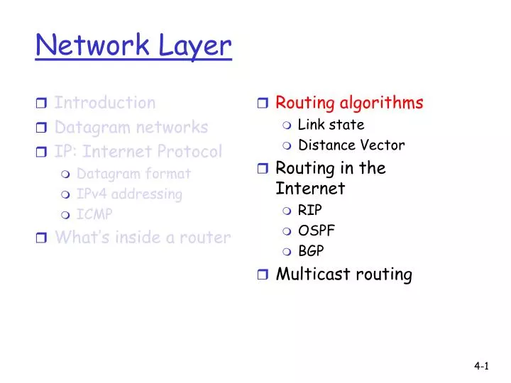
Introduction Datagram networks IP: Internet Protocol Datagram format IPv4 addressing ICMP What’s inside a router. Routing algorithms Link state Distance Vector Routing in the Internet RIP OSPF BGP Multicast routing. Network Layer. routing algorithm. local forwarding table.

E N D
Introduction Datagram networks IP: Internet Protocol Datagram format IPv4 addressing ICMP What’s inside a router Routing algorithms Link state Distance Vector Routing in the Internet RIP OSPF BGP Multicast routing Network Layer
routing algorithm local forwarding table header value output link 0100 0101 0111 1001 3 2 2 1 value in arriving packet’s header 1 0111 2 3 Interplay between routing and forwarding [1] Fact: Forwarding is based on a forwarding/routing table. [2] Question: how do we build up the routing table? Answer: routing alg.
5 3 5 2 2 1 3 1 2 1 x z w u y v Graph abstraction Graph: G = (N,E) N = set of routers = { u, v, w, x, y, z } E = set of links ={ (u,v), (u,x), (v,x), (v,w), (x,w), (x,y), (w,y), (w,z), (y,z) } Remark: Graph abstraction is useful in other network contexts Example: P2P, where N is set of peers and E is set of TCP connections
5 3 5 2 2 1 3 1 2 1 x z w u y v Graph abstraction: costs • c(x,x’) = cost of link (x,x’) • - e.g., c(w,z) = 5 • cost could always be 1, or • inversely related to bandwidth, • or inversely related to • congestion Cost of path (x1, x2, x3,…, xp) = c(x1,x2) + c(x2,x3) + … + c(xp-1,xp) Question: What’s the least-cost path between u and z ? Routing algorithm: algorithm that finds least-cost path
Global or decentralized information? Global: all routers have complete topology, link cost info “link state” algorithms Decentralized: router knows physically-connected neighbors, link costs to neighbors iterative process of computation, exchange of info with neighbors “distance vector” algorithms Static or dynamic? Static: routes change slowly over time Dynamic: routes change more quickly periodic update in response to topology or link cost changes Routing Algorithm classification
Introduction Datagram networks IP: Internet Protocol Datagram format IPv4 addressing ICMP What’s inside a router Routing algorithms Link state Distance Vector Routing in the Internet RIP OSPF BGP Multicast routing Network Layer
Dijkstra’s algorithm net topology, link costs known to all nodes accomplished via “link state broadcast” all nodes have same info computes least cost paths from one node (‘source”) to all other nodes gives forwarding table for that node iterative: after k iterations, know least cost path to k dests Notation: c(x,y): link cost from node x to y; = ∞ if not direct neighbors D(v): current value of cost of path from source to dest. v p(v): predecessor node along path from source to v N': set of nodes whose least cost path definitively known A Link-State Routing Algorithm
The Link State Packet includes: The ID of the router that created the LSP List of directly connected neighbors, and cost Sequence number TTL Reliable Flooding Resend LSP over all links other than incident link, if the sequence number is newer. Otherwise drop it. Link State Detection: Link layer failure Loss of “hello” packets Reliable Flooding of LSP
Dijsktra’s Algorithm 1 Initialization: 2 N' = {u} 3 for all nodes v 4 if v adjacent to u 5 then D(v) = c(u,v) 6 else D(v) = ∞ 7 8 Loop 9 find w not in N' such that D(w) is a minimum 10 add w to N' 11 update D(v) for all v adjacent to w and not in N' : 12 D(v) = min( D(v), D(w) + c(w,v) ) 13 /* new cost to v is either old cost to v or known 14 shortest path cost to w plus cost from w to v */ 15 until all nodes in N'
5 3 5 2 2 1 3 1 2 1 x z w y u v Dijkstra’s algorithm: example D(v),p(v) 2,u 2,u 2,u D(x),p(x) 1,u D(w),p(w) 5,u 4,x 3,y 3,y D(y),p(y) ∞ 2,x Step 0 1 2 3 4 5 N' u ux uxy uxyv uxyvw uxyvwz D(z),p(z) ∞ ∞ 4,y 4,y 4,y
x z w u y v destination link (u,v) v (u,x) x y (u,x) (u,x) w z (u,x) Dijkstra’s algorithm: example (2) Resulting shortest-path tree from u: Resulting forwarding table in u:
Algorithm complexity: n nodes each iteration: need to check all nodes, w, not in N n(n+1)/2 comparisons: O(n2) more efficient implementations possible: O(nlogn) Oscillations possible: e.g., link cost = amount of carried traffic A A A A D D D D B B B B C C C C 1 1+e 2+e 0 2+e 0 2+e 0 0 0 1 1+e 0 0 1 1+e e 0 0 0 e 1 1+e 0 1 1 e … recompute … recompute routing … recompute initially Dijkstra’s algorithm, discussion
Introduction Datagram networks IP: Internet Protocol Datagram format IPv4 addressing ICMP What’s inside a router Routing algorithms Link state Distance Vector Routing in the Internet RIP OSPF BGP Multicast routing Network Layer
Distance Vector Algorithm Bellman-Ford Equation (dynamic programming) Define dx(y) := cost of least-cost path from x to y Then dx(y) = min {c(x,v) + dv(y) } where min is taken over all neighbors v of x v
5 3 5 2 2 1 3 1 2 1 x z w u y v Bellman-Ford example Clearly, dv(z) = 5, dx(z) = 3, dw(z) = 3 B-F equation says: du(z) = min { c(u,v) + dv(z), c(u,x) + dx(z), c(u,w) + dw(z) } = min {2 + 5, 1 + 3, 5 + 3} = 4 Node that achieves minimum is next hop in shortest path ➜ forwarding table
Distance Vector Algorithm • Dx(y) = estimate of least cost from x to y • Distance vector: Dx = [Dx(y): y є N ] • Node x knows cost to each neighbor v: c(x,v) • Node x maintains Dx = [Dx(y): y є N ] • Node x also maintains its neighbors’ distance vectors • For each neighbor v, x maintains Dv = [Dv(y): y є N ]
Distance vector algorithm (4) Basic idea: • Each node periodically sends its own distance vector estimate to neighbors • When a node x receives new DV estimate from neighbor, it updates its own DV using B-F equation: Dx(y) ← minv{c(x,v) + Dv(y)} for each node y ∊ N • Under minor, natural conditions, the estimate Dx(y) converge to the actual least cost dx(y)
Iterative, asynchronous: each local iteration caused by: local link cost change DV update message from neighbor Distributed: each node notifies neighbors only when its DV changes neighbors then notify their neighbors if necessary wait for (change in local link cost of msg from neighbor) recompute estimates if DV to any dest has changed, notify neighbors Distance Vector Algorithm (5) Each node:
cost to x y z x 0 2 7 y from ∞ ∞ ∞ z ∞ ∞ ∞ 2 1 7 z x y Dx(z) = min{c(x,y) + Dy(z), c(x,z) + Dz(z)} = min{2+1 , 7+0} = 3 Dx(y) = min{c(x,y) + Dy(y), c(x,z) + Dz(y)} = min{2+0 , 7+1} = 2 node x table cost to cost to x y z x y z x 0 2 3 x 0 2 3 y from 2 0 1 y from 2 0 1 z 7 1 0 z 3 1 0 node y table cost to cost to cost to x y z x y z x y z x ∞ ∞ x 0 2 7 ∞ 2 0 1 x 0 2 3 y y from 2 0 1 y from from 2 0 1 z z ∞ ∞ ∞ 7 1 0 z 3 1 0 node z table cost to cost to cost to x y z x y z x y z x 0 2 7 x 0 2 3 x ∞ ∞ ∞ y y 2 0 1 from from y 2 0 1 from ∞ ∞ ∞ z z z 3 1 0 3 1 0 7 1 0 time
1 4 1 50 x z y Distance Vector: link cost changes Link cost changes: • node detects local link cost change • updates routing info, recalculates distance vector • if DV changes, notify neighbors At time t0, y detects the link-cost change, updates its DV, and informs its neighbors. At time t1, z receives the update from y and updates its table. It computes a new least cost to x and sends its neighbors its DV. At time t2, y receives z’s update and updates its distance table. y’s least costs do not change and hence y does not send any message to z. “good news travels fast”
Bellman-Ford Algorithm Questions: • How long can the algorithm take to run? • How do we know that the algorithm always converges? • What happens when link costs change, or when routers/links fail? Topology changes make life hard for the Bellman-Ford algorithm…
A Problem with Bellman-Ford “Bad news travels slowly” 1 1 1 R1 R2 R3 R4 Consider the calculation of distances to R4: Time R1 R2 R3 0 3,R2 2,R3 1, R4 R3 R4 fails 1 3,R2 2,R3 3,R2 2 3,R2 4,R3 3,R2 3 5,R2 4,R3 5,R2 … … … … “Counting to infinity”
Set infinity = “some small integer” (e.g. 16). Stop when count = 16. Split Horizon: Because R2 received lowest cost path from R3, it does not advertise cost to R3 Split-horizon with poison reverse: R2 advertises infinity to R3 R2 gets to R4 thru R3 There are many problems with (and fixes for) the Bellman-Ford algorithm. Counting to Infinity ProblemSolutions
Message complexity LS: with n nodes, E links, O(nE) msgs sent DV: exchange between neighbors only convergence time varies Speed of Convergence LS: O(n2) algorithm requires O(nE) msgs may have oscillations DV: convergence time varies may be routing loops count-to-infinity problem Robustness: what happens if router malfunctions? LS: node can advertise incorrect link cost each node computes only its own table DV: DV node can advertise incorrect path cost each node’s table used by others error propagate thru network Comparison of LS and DV algorithms
Space requirement LS: Maintain entire topology DV: Maintain only neighbor state Comparison of LS and DV algorithms