Download
1 / 34
340 likes | 441 Vues
EFW Science Overview. Professor John R. Wygant (PI) University of Minnesota. Level-1 Mission Science Goals.

E N D
EFW Science Overview Professor John R. Wygant (PI) University of Minnesota
Level-1 Mission Science Goals Provide understanding, ideally to the point of predictability of how populations of relativistic electrons and penetrating ions in space form or change in response to variable input from the sun Which physical processes produce radiation enhancement events? What are the dominant processes for relativistic electron loss? How do ring current and other geomagnetic processes affect radiation belt behavior? EFW measures DC electric fields, density, and waves responsible for the accelerations, loss, and structure of energetic charged particles
Level-1 Science ObjectivesEFW Measurements The RBSP mission will determine local steady and impulsive electric and magnetic fields …These products will enable the the scientific goals of determining convective and impulsive flows, determining properties of shock generated shock fronts… The RBSP mission will derive and determine spatial and temporal variations of electrostatic and electromagnetic field amplitudes, frequency, intensity, propagation direction, spatial distribution and temporal evolution with sufficient fidelity to calculate wave energy, polarization, saturation levels, coherence, wave normal angle, phase velocity, and wave number for a) VLF and ELF waves, and b) random, ULF, and quasi-periodic electromagnetic fluctuations. These products will enable the scientific goals of determining the types and characteristics of plasma waves causing particle energization and loss including wave growth rates; quantifying adiabatic and non-adiabatic mechanisms of energization and loss........; determining conditions that control the production and propagation of waves High time resolution burst electric and magnetic fild measurements will provide understanding of the role in the prompt acceleration and loss of energetic particles of non-linear interactions with discrete large amplitude wave structures.
EFW Instrument Overview +Z • RBSP EFW Features • Four spin plane booms (2 x 40 m and 2x 50 m) • Two spin axis stacer booms (2x6 m) • Spherical sensors and preamplifiers near outboard tip of boom (400 kHz response) • Flexible boom cable to power sensor electronics & return signals back to SC • Sensors are current biased by instrument command to be within ~ 1 volt of ambient plasma potential. • Main electronic box (sensor bias control filtering, A-D conversion, burst memory, diagnostics, mode commanding, TM formatting ) • EFW Science quantities include: • • E-fields:(V1-V2, V3-V4, V5-V6) • Interferometric timing: SC-sensor potential (V1s, V2s, V3s, V4s, V5s, V6s) • SC Potential : (V1+V2)/2, (V3+V4)/2 • Interface to EMFISIS instrument • Electrostatic cleanliness spec: variations of potential across spacecraft surfaces smaller than 1 Volt. 2 5 4 3 6 Not to Scale 1
Cut-Away Mechanisms associated with energetic particle acceleration and transport (B. Mauk/APL)
Level-1 Science and Measurement Objectives (1) • Science Objective: Measure electric fields associated with a variety of mechanisms “causing particle energization and scattering” in the inner magnetosphere. • These mechanisms include: • Energization by the large-scale “steady state and storm time convection E-field” . • Energization by substorm “transient fronts”propagating in from the tail. • “Radial diffusion of energetic particles” mediated by “ULF waves”. • Transport and energization by interplanetary “shock generated transient fronts.” • Adiabatic and non-adiabatic energization by “electromagnetic and electrostatic” waves and (“random”) structures .
CRRES measurements of the E-field during a pass through the inner magnetosphere: interplanetary shock induced electric field, large scale MHD waves, and enhancement in convection electric field. E-Fields in the Active Radiation Belt MHD waves: an important mechanism for radially diffusing and energizing particles. The shock induced magnetosonic wave created a 5 order of magnitude increase in 13 MeV electron fluxes in <100 seconds resulting in a new radiation belt that lasted two years The large scale electric field produced a ~70 kV potential drop between L=2 & L-4 and injected ring current plasma. dDst/dt= - 40 nT/hr
EFW Targeted Energization/Transport Mechanisms and Structures
Primary Measurement Requirements Flow to Instrument
Electric Fields & WavesDriving Requirements Spin plane component of E-field at DC-15 Hz (>0.3 mV/m or 10% sensitivity) over a range from 0 to 500 mV/m at R>3.5 Re …(IPLD 38) Spin axis component of E at DC-15 Hz (>4 mV/m or 20% sensitivity) over a range from 2-500 mV/m at R>3.5Re (IPLD 44) Spacecraft potential measurements providing estimates of cold plasma densities of 0.1 to ~50 cm-3 at 1-s cadence (dn/n<50%) (IPLD 55) Programmable high time resolutions burst recordings of large amplitude (Req.: 0.4 -500 mV/m capability: 0-4V/m) E-fields ; B-fields and cold electron density variations 0.1-50 cm-3 with sensitivity of 10% (derived from SC potential) over frequency range from dc to 250 Hz (IPLD 42,47,71, 59) Burst Interferometric timing of intense (0.1-300mV/m) small scale electric field structures and non-linear waves: timing accuracy of .06 ms for velocities of structures over 0-500 km/s (IPLD 61) Broad Band Filters (8 freq bins-peak or average) power in wave electric field at 8 samples/s. Burst Triggers/Selection Diagnostic; Solitary Wave Counter: Burst Diagnostic (IPLD 42,47,71,59,61) Spectra & Cross Spectra of average/peak electric and magnetic fluctuations from 1 Hz to 300 Hzwith a cadence of 1/8 seconds over a range 80 dB as a diagnostic of large amplitude wave properties over orbital scales. (IPLD 66,68). Low noise 3-D E-field waveforms to EMFISIS: 10 Hz to 400 kHz; maximum signal 30 mV/m. For spin plane sensors: range of 100 dB & sensitivities of 3 x 10-14 V2/m2Hz at 1 kHz and 3 x 10-17 V2/m2Hz at 100 kHz. For spin axis sensor pairs: range x 10 less & sensitivity x 100 less (IPLD 245, 246)
Observations of large amplitude turbulent electric fields E~+/-500 mV/m Duration of spike 20-200 Hz Polarized perpendicular to B B~0.5 nT (not shown) Hodograms for E and B Complicated quasi 3D structure full 3D and 3DB Waves electrostatic with phase fronts ~perp to B Large amplitude thermal plasma variations measured from SC potential variations:Result in order of magnitude changes in index of refraction wave time scales: trapping motivates SC potential measurements Position R=5.2, Mlat 25 deg, MLT=0.5 Observed during nearly conjugate ~400 keV electron microburst interval by low altitude SAMPEX. Polar Observations of Intense Waves Motivating High Time Resolution Burst Measurements
EFW Burst Modes 1 and 2 In order to obtain high time resolution measurements of small scale waves and structures and not exceed its TM allocation the EFW instrument has two Bursts Modes with different memories and different means of selecting and playing back data: Burst 1: Nominal sampling 512 samples/s of 3D E-field and 3D Search Coil (from EMFISIS), Spacecraft Potential Density (Thermal Plasma Fluctuations). 32 Gigabytes of Memory. Filled in ~40 days. During TM contacts low rate survey data is sent to ground. Then over several days survey data is evaluated by EFW scientist for time intervals of substorm injections, shocks, and other structures driving waves. Desired burst times and priority are up-linked and the instrument forms a queue and sends data down. Autonomous modes and commanded time tagged triggers available. (7.5% duty cycle) 2) Burst 2: Interferometric Timing Measurements from Single ended measurements. (6.5 kHz time resolution). Autonomously triggered off large amplitude excursions using on board signals from DCB (~200 Mbytes). Bursts placed in queue on basis of “best trigger quality” and best played first. No human intervention (0.1% duty cycle) Diagnostic context for burst data over orbital scales is provided by spectra and cross spectra of E and B, broad band filters/peak detectors, and solitary wave counters. Information on burst status is provided to other instruments via burst status word via Spacecraft
Functional Block Diagram Potential of sensor relative to SC measured with high input impedance preamplifier near sensor. Current biasing of sensors controls operating point on I/V curve of sphere-plasma sheath decreasing source impedance by 2 orders of magnitude and fixes floating potential of sphere Voltage biasing of surfaces of preamplifier housing (guard and usher) controls flow of photo-current to sensor from booms and housing- decreasing major error source Thin wire to sphere has small surface area--further decreases photo-electrons error source. Pre-amplifier near sphere drives for long cable. Sets 400 kHz freq response of high frequency signal to EMFISIS. Boom Electronics Board (BEB) provides bias signals, power to sensor via cable . Receives E-field signals from 6 sensors.Tranfers signals to Digitial Filter Board in our instrument. Sends 3 differential E-field signals to the EMFISIS instrument (10 Hz to 400 kHz). Digital Filter Board (DFB): analog circuitry create differential signals and high frequency (6.5 kHz)anti-aliasing filtering. Receives Search Coil (1 -250 Hz) and Flux gate signals (dc -10 Hz from EMFISIS (3 signals). All Signals sampled by two 16 bit A-D converters providing sufficient dynamic range. Lower Frequency Nyquist Filtering done by algorithms implemented in FPGA on DFB. E and B Spectra, and Cross Spectra between E and B are provided by DFB as context for burst wave forms. Fast Broad Band Filters provide triggers for Bursts and a further high time resolution context.
Functional Block Diagram (2) Digital Control Board: Commands current and voltage biasing of sensors by BEB Controls DFB sampling formats, filtering, rates. Commands DFB spectra & cross-spectra calculations Controls triggering, storing, and play back of high time resolution burst data in SDRAM and large Flash memory. Supports human selected burst, bursts autonomously triggered by large amplitude signals, and time-tagged bursts. Spin fits from probes provide high quality 2 D electric field vector (removes offsets) in spin plane. This is an input to space weather and provides high quality E-field survey data for burst selection on ground. Supports compression, formating, and transfer of science data to spacecraft. A variety of other engineering functions discussed in detail by Ludlam, Gordon, and Harvey
EFW Space Weather Data Products(IPLD 574) EFW will provide: 2D Spin Plane Vector Electric Field Cadence: 1 vector/spin (~12 sec) 2 components in despun coordinates Spacecraft Potential (estimate of cold plasma density) 1 scalar per spin (12 sec) Involves on board calculation implemented on previous spacecraft 28 bytes/12 s spin gives 18.66b/s of SWX bit-rate
Time Duration of Intervals of Low Frequency Bursting Necessary for Understanding Wave Fields Responsible for Scattering/Acceleration of Energetic Particles In order to obtain this data, we must have a burst memory of sufficient size, adequate telemetry to downlink the data,and a strategy for selecting the appropriate time intervals
Spin Plane Electric Field Measurement STARD Requirement at different altitudes including validity requirement
Spin Plane Deployment, Partially Deployed Cable, Pre-Amplifier Housing, Thin Wire, and Sphere
Measured and model average large scale convection electric field in inner magnetosphere. Traces are for different values of geomagnetic activity. Kp varies: 1-8. Quiet time field accurate to <0.2 mV/m. RBSP ~twice as accurate. Requirement is larger of either <0.3 mV/m or 10% of magnitude of E for Radial distance > 3.5 Re. CRRES accuracy of large scale electric field measurement on spacecraft comparable to RBSP after ground calibration
Discussion of accuracy of VxB subtraction •Since the SC is moving relative to the Earth there is a motional electric field V xB where V is the spacecraft velocity and B is the measured magnetic field of the Earth which must be subtracted from the measured electric field in order to determine the electric field in the rest frame of the Earth. • Angular uncertainties in the attitude of the spacecraft or orientation of electric field or magnetic field or determination of spacecraft velocity measurements create errors in the electric field which must obey MRD/ELE 42. • Plots of typical motional electric field and uncertainties in the measured electric field for 1deg and 3 deg attitude errors as a function of radial distance for an ensemble of orbits is presented in the next slide • Required limits on angular error are defined in the subsequent slide • All errors are at the 3 sigma level • Time independent errors can be reduced signficantly (factor of 2-3) by on the ground cross calibration of the measured electric field and V x B for quiet time orbits as indicated by CRRES experience. Time independent errors are dominant contributions to the magnetometer boom angular uncertainties and electric field sensor alignment uncertainties. • CRRES was able to achieve an accuracy of ~ 0.1 mV/m after somewhat extensive ground calibration. This calibration is part of “scientific analysis”. The present RBSP EFW requirement is 0.3 mV/m at a distance of 3.5 Re. CRRES pointing accuracies were less stringent than RBSP.
Aspects of alignment calibration The magnetic field measurement compared to the magnetic field will provide a strong constraint on the alignment of the spacecraft within a rotation angle arround the magnetic field This angle can be constrained by comparison of the measured E to VxB during geomagnetically quite times Kp<2. The orthogonality of the V12 and V34 boom pairs can be constrained by using time intervals when VxB has a significant component in the spin plane. The sine waves measured by the rotating orthogonal booms pairs should be 90 degrees out of phase. Comparison of amplitudes of the sine waves to projection of VxB into spin plane provides calibration of magnitude. We can also use the 40m and 50 m boom baseline difference to calibrate the electric field magnitude. Attitude manveuvers will take place event ~27 days. After the attitude maneuvers it is possible that the sun pulse will provide the most accuracy attitude measurement. Since the sun sensor is most accurate when the spin axis points away from the sun. Many calibrations of time independent boom alignment error quantities are best preformed at these times.
Contributions to E field accuracy of transformation from spacecraft frame to inertial GSE frame E= Em-VxB Blue high light are dominate contributions
Effect of Attitude Uncertainty in E-VxB subtraction accuracy
1000 Large Amplitude Alfven Wave at PSBL with imbedded large amplitude LH “type” waves R=5.2 Re, 0.82 MLT, MLAT~25 deg Ez ~300 mV/m By~100 nT Propagate parallel to B tpwards Earth Vphase~ 3000-10000 km/s E-Field (mV/m) (~800 Hz) 0 25 duration burst Z GSM -1000 100 50 B-Field (nT) Y GSM Low freq (8 Hz) Notice:Imbedded bursts of high frequency waves ~1 V/m ptp (greater in other components) 0
SAMPEX in low altitude orbit encounters outer radiation belts ~10 minutes after Polar about 1 hour in MLT distant SAMPEX observes rapid time variations (0.1-1 seconds) in 500 keV electron fluxes Fluxes vary by almost order of magnitude Consistent with strong scattering of electrons due to waves (similar to Cattell et al. this meeting) Coincides with Polar L-value
EFW – PRE, BEB, EFW-EMFMotivation (In Words) The EFW Sensors, Preamp, BEB and EFW-EMFISIS interface represent the primary analog signal path for E-field measurements on RBSP. Measuring 0.1 mV/m DC E-fields required accuracies of 0.1% in the magnetosphere: tens of mV of signal in the presence of tens to hundreds of mV/m of effective common-mode or systematic noise (photocurrents, SC charging), or tens of volts of common mode signal. Non-linear coupling (I-V curve) of EFW sensors to E-field can be optimized through current biasing (factor of 100 decrease in susceptibility to systematic error sources and density fluctuations). Current biasing of sensors drives volts to tens of volts floating potential differences between sensors and SC ground. High effective source impedance (plasma sheath, ten of MΩ), and low-noise and low-leakage current requirements (systematic error reduction again) drive use of low-voltage preamps in floating ground configuration. Deflection and collection of stray photoelectron currents prior to impingement upon sensor also reduces DC biases (WHIP/USHER and GUARD surfaces).
EFW – PRE, BEB, EFW-EMFPerformance Requirements Formal requirements presented in SysEng presentation. Informally: Measure few tenths of mV/m to few hundreds of mV/m 2D DC E-fields associated with global convection, ULF waves, and shock-driven effects (spin plane). Measure few few mV/m to few hundreds of mV/m 3D DC E-fields (spin plane and spin axis) associated with same. Measure 3D E-field fluctuations up to a 6 kHz at amplitudes up to hundreds of mV/m associated with energetic electron acceleration, scattering and transport. Deliver low-noise analog E-field signals to EMFISIS-WAVES from 10 Hz to 400 kHz to allow for measurement of tens of mV/m E-field fluctuations associated with energetic electron acceleration, scattering, and transport, as well as detection of the upper hybrid line for cold plasma density estimation. Measure SC potential fluctuations associated with quasi-DC and low-frequency plasma density and fluctuations. These measurement requirements drive the design of the Preamp, the Boom Electronics Board (BEB) and EFW-EMFISIS E-Field interface.
EFW – PRE, BEB, EFW-EMFMotivation (In Pictures) Sensor I-V curve and sheath impedance Sensor and SC Floating Potentials SC Sensors photoelectrons ambient e- photo e- plasma e-