Download
1 / 12
150 likes | 193 Vues
EE 351M Digital Signal Processing Fall 2015. Sampling and Aliasing. Prof. Brian L. Evans Dept. of Electrical and Computer Engineering The University of Texas at Austin. Please join me for coffee hours on Fridays 12-2pm in fall and spring semesters. Outline.

E N D
EE 351M Digital Signal Processing Fall 2015 Sampling and Aliasing Prof. Brian L. Evans Dept. of Electrical and Computer Engineering The University of Texas at Austin Please join me for coffeehours on Fridays 12-2pmin fall and spring semesters
Outline • Data conversion • Sampling Time and frequency domains Sampling theorem • Aliasing • Bandpass sampling • Conclusion
Data Conversion Analog Lowpass Filter Quantizer Sampler at sampling rate of fs Discrete to Continuous Conversion Analog Lowpass Filter fs Data Conversion • Analog-to-Digital Conversion Lowpass filter hasstopband frequencyless than ½ fs to reducealiasing due to sampling(enforce sampling theorem) • Digital-to-Analog Conversion Discrete-to-continuousconversion could be assimple as sample and hold Lowpass filter has stopbandfrequency less than ½ fs reduce artificial high frequencies
Sampling - Review Sampling: Time Domain • Many signals originate in continuous-time Talking on cell phone, or playing acoustic music • By sampling a continuous-time signal at isolated, equally-spaced points in time, we obtain a sequence of numbers n {…, -2, -1, 0, 1, 2,…} Ts is the sampling period. Ts t Ts f(t) Sampled analog waveform impulse train
Sampling - Review F(w) G(w) w w -2pfmax 2pfmax -ws ws -2ws 2ws Sampling: Frequency Domain • Sampling replicates spectrum of continuous-time signal at integer multiples of sampling frequency • Fourier series of impulse train where ws = 2 pfs Modulationby cos(2 s t) Modulationby cos(s t) How to recover F()?
Sampling - Review Sampling Theorem • Continuous-time signal x(t) with frequencies no higher than fmax can be reconstructed from its samples x(n Ts) if samples taken at rate fs > 2 fmax Nyquist rate = 2 fmax Nyquist frequency = fs / 2 • Example: Sampling audio signals Normal human hearing is from about 20 Hz to 20 kHz Apply lowpass filter before sampling to pass low frequencies up to 20 kHz and reject high frequencies Lowpass filter needs 10% of maximum passband frequency to roll off to zero (2 kHz rolloff in this case)
Sampling Sampling a Cosine Signal • Sample a cosine signal of frequency f0 in Hz x(t) = cos(2 f0t) Sample at rate fs > 2 f0 by substituting t = nTs = n / fs x[n] = cos(2 f0 (n / fs)) = cos(2 (f0 / fs) n) • Discrete-time frequency 0 = 2 f0 / fsin units of rad/sample With f0 = 1200 Hz and fs = 8000 Hz, 0 = 3/10 rad/sample • Discrete-time cosine with frequency 0 x[n] = cos(ω0n)
Sampling Sampling and Oversampling • As sampling rate increases above Nyquist rate, sampled waveform looks more like original • Zero crossings: frequency content of a sinusoid Distance between two zero crossings: one half period With sampling theorem satisfied, sampled sinusoid crosses zero right number of times per period In some applications, frequency content matters not time-domain waveform shape • DSP First, Ch. 4, Sampling/Interpolation demo For username/password help link link
Continuous-time sinusoid x(t) = A cos(2p f0 t+ f) Sample at Ts = 1/fs x[n] = x(Tsn) =A cos(2p f0 Ts n + f) Keeping the sampling period same, sample y(t) = A cos(2p (f0 + l fs) t + f) where l is an integer y[n] = y(Tsn) = A cos(2p(f0 + lfs)Tsn + f) = A cos(2pf0Tsn + 2plfsTsn + f) = A cos(2pf0Tsn + 2pln + f) = A cos(2pf0Tsn + f) = x[n] Here, fsTs = 1 Since l is an integer,cos(x + 2 p l) = cos(x) y[n] indistinguishable from x[n] Aliasing Aliasing
Bandpass Sampling Ideal Bandpass Spectrum f –f1 f2 –f2 f1 Sampled Ideal Bandpass Spectrum f –f1 f2 –f2 f1 Bandpass Sampling • Reduce sampling rate Bandwidth: f2 – f1 Sampling rate fs mustbe greater than analogbandwidth fs > f2 – f1 For replica to be centeredat origin after samplingfcenter = ½(f1 + f2) = kfs • Practical issues Sampling clock tolerance: fcenter = kfs Effects of noise Sample atfs Lowpass filter to extract baseband
Bandpass Sampling Upconversion method Sampling plus bandpass filtering to extract intermediate frequency (IF) band with fIF = kIFfs Downconversion method Bandpass sampling plus bandpass filtering to extract intermediate frequency (IF) band with fIF = kIFfs f f Sample atfs -fmax fmax –f1 f2 –f2 f1 f -fIF -fs fs fIF Sampling for Up/Downconversion f –f1 -fIF –f2 fIF
Conclusion Conclusion • Sampling replicates spectrum of continuous-time signal at offsets that are integer multiples of sampling frequency • Sampling theorem gives necessary condition to reconstruct the continuous-time signal from its samples, but does not say how to do it • Aliasing occurs due to sampling • Bandpass sampling reduces sampling rate significantly by using aliasing to our benefit