Download
1 / 35
350 likes | 482 Vues
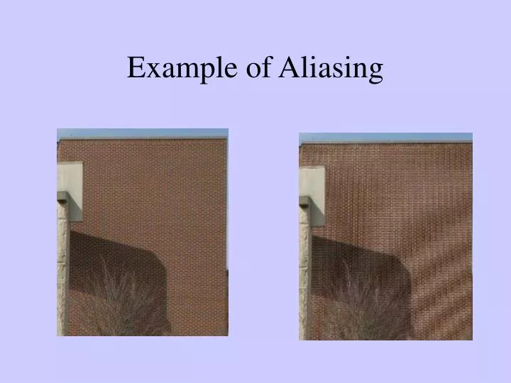
Example of Aliasing. Sampling and Aliasing in Digital Images. Array of detector elements Sampling (pixel) pitch Detector aperture width The spacing between samples determines the highest frequency that can be imaged Nyquist frequency: F N = 1/2 D

E N D
Sampling and Aliasing in Digital Images • Array of detector elements • Sampling (pixel) pitch • Detector aperture width • The spacing between samples determines the highest frequency that can be imaged • Nyquist frequency: FN = 1/2D • If a frequency component in an image > FN → sampled < 2x/cycle: aliasing • Wraps back into the image as a lower frequency • Moiré pattern, spoke wheels c.f. Bushberg, et al. The Essential Physics of Medical Imaging, 2nd ed., p. 284.
Sampling and Aliasing in Digital Images • Example: sampling pitch of 100 mm → FN = 5 cycles/mm When input f > FN then the spatial frequency domain signal at f is aliased down to: • fa = 2FN– f • Not noticeable with patient • Antiscatter grids • Aperture blurring - signal averaging across the detector aperture c.f. Bushberg, et al. The Essential Physics of Medical Imaging, 2nd ed., pp. 285-286.
Noise is anything in the image that is not the signal we are interested in seeing. • Noise can be structured or Random.
Structure Noise Noise which comes from some non-random source: breast parenchyma, hum bars in CRT’s. The design goal in making an imaging system is to reduce structure or system noise to below the level of the random noise.
Random or Quantum Noise Noise resulting from the statistical nature of the signal source is random or quantum noise. • In imaging, the signal is light in the form of photons being emitted randomly in time and space. • Because we are working with a random source, we can use statistics to describe the behavior of the image noise.
Rose Model • The information content of a finite amount of light is limited by the finite number of photons, by the random character of their distribution, and by the need to avoid false alarms (false positives). • The measure of how well an object (signal) can be seen against a background of varying signal strength (noise) is the signal to noise ratio: S/N.
Rose Model • To see an object of a given diameter (resolution) you must have sufficient contrast and S/N. • In an ideal system, where the only noise is quantum noise, the diameter, D, which can be resolved is given by: • D2 x n2 = k2/C2 where C is the contrast of the detail, n is the number of photons/sq cm in the image, and k is the threshold S/N ratio. • Most people use k=5. • (remember, good resolution means D is small)
Contrast Resolution • Ability to detect a low-contrast object Related to how much noise there is in the image → SNR • As SNR ↑ the CR ↑ • Rose criterion: SNR > 5 to reliably identify an object • Quantum noise and structure noise both affect the conspicuity of a target c.f. Bushberg, et al. The Essential Physics of Medical Imaging, 2nd ed., p. 281.
Gaussian Probability Distribution Function • Gaussian (normal) distribution: <X> the mean • and σ describe the shape • Many commonly encountered measurements of people and things make for this kind of distribution (Gaussian) hence the term “normal” e.g., the height of 1000 third grade school children approximates a Gaussian c.f. Bushberg, et al. The Essential Physics of Medical Imaging, 2nd ed., p. 275.
MEAN Xi X = i N VARIANCE ( Xi - X )2 2 = i (N - 1) FOR GAUSSIAN PROBABILITY DISTRIBUTION
STANDARD DEVIATION ~ 2 = = X FOR GAUSSIAN PROBABILITY DISTRIBUTION
ASSUMPTIONS FOR A NORMAL PROBABILITY DISTRIBUTION • SAMPLE SELECTED FROM A LARGE POPULATION • SAMPLE = HOMOGENEOUS • STOCHASTIC = RANDOM MEASUREMENT PROCESS • NO SYSTEMATIC ERRORS AFFECTING THE RESULTS
GAUSSIAN (NORMAL) STATISTICAL DISTRIBUTIONS • MEAN - 1 STD < X < MEAN + 1 STD • CONTAINS 68.3 % OF MEASUREMENTS • MEAN - 2 STD < X < MEAN + 2 STD • CONTAINS 95.5 % OF MEASURMENTS • MEAN - 3 STD < X < MEAN + 3 STD • CONTAINS 99.7 % OF MEASUREMENTS
Poisson Probability Distribution Function • Poisson distribution: • m = mean, shape governed by one variable • P(x) difficult to calculate for large values of x due to x! • X-ray and g-ray counting statistics obey P(x) • Used to describe • Radioactive decay • Quantum mottle
Probability Distribution Functions • Probability of observing an observation in a range: integrate area (for G): • 1 σ = 68.25% • 1.96 σ = 95% • 2.58 σ = 99% • Error bars and confidence intervals • P(x) very similar to G(x) when σ ≈ √x → use G(x) as approx. • Can adjust the noise (σ) in an image by adjusting the mean number of photons used to produce the image c.f. Bushberg, et al. The Essential Physics of Medical Imaging, 2nd ed., pp. 276 - 277.
GAUSSIAN (NORMAL) DISTRIBUTION EXP[ - ( X - X ) 2 / 2 2 ] (2 )0.5
0.14 0.12 0.1 0.08 PROBABILITY OF RESULT 0.06 0.04 0.02 0 0 5 10 15 20 25 30 35 40 45 NUMBER OF HEADS BINOMIAL POISSON GAUSSIAN COMPARISON OF VARIOUS STATISTICAL DISTRIBUTIONS OF PROBABILITY FOR COIN FLIPPING
Quantum Noise • N = mean photons/unit area • σ = √N, from P(x) → σ2 (variance) = N • Relative noise = coefficient of variation = σ/N = 1/√N (↓ with ↑ N) • SNR = signal/noise = N/σ = N/√N = √N (↑ with ↑ N) • Trade-off between SNR and radiation dose: SNR ↑ 2x → Dose ↑ 4x c.f. Bushberg, et al. The Essential Physics of Medical Imaging, 2nd ed., p. 278.
Noise Frequency: the Wiener Spectrum W(f) • Although noise appears random, the noise has a frequency distribution • Example: ocean waves • Take a flat-field x-ray image (still has noise variations) Fourier Transform (FT) the flat image → Noise Power Spectrum: NPS(f) NPS(f) is the noise variance (σ2) of the image expressed as a function of spatial freq. (f) c.f. Bushberg, et al. The Essential Physics of Medical Imaging, 2nd ed., p. 282.
Detective Quantum Efficiency • DQE: metric describing overall system SNR performance and dose efficiency • DQE = • SNR2in = N (→ SNR = √N) • SNR2out = • DQE(f) = DQE(f=0) = QDE c.f. Bushberg, et al. The Essential Physics of Medical Imaging, 2nd ed., p. 282.
Contrast Detail (C-D) Curves • Spatial resolution: MTF(f) • Contrast resolution: SNR • Combined quantitative: DQE(f) • Qualitative: C-D curve • C-D phantom: holes in plastic of ↓ depth and diameter • What depth hole at which diameter can just be visualized • Connect the dots → C-D line • Better spatial resolution: high-contrast, small detail • Better contrast resolution: low-contrast c.f. Bushberg, et al. The Essential Physics of Medical Imaging, 2nd ed., p. 287.
Receiver Operating Characteristic Curves • The ROC curve is essentially a way of analyzing the SNR associated with a specific diagnostic task Az: area under the curve – concise description of the diagnostic performance of the systems (including observers) being tested • Measure of detectability • Az = 0.5 guessing • Az = 1.0 perfect c.f. Bushberg, et al. The Essential Physics of Medical Imaging, 2nd ed., p. 291.
Receiver Operating Characteristic Curves • Diagnostic task: separate abnormal from normal • Usually significant overlap in histograms • Decision criterion or threshold • Based on threshold: either normal (L) or abnormal (R) • N cases: 2 x 2 decision matrix • TPF= TP/(TP+FN)= Sensitivity • FPF = FP/(FP+TN) • Specificity = (1-FPF) = TNF • ROC curve: sensitivity vs. 1-specificity usu. @ five threshold levels c.f. Bushberg, et al. The Essential Physics of Medical Imaging, 2nd ed., pp. 288-289.
The ROC Cookbook Rank Signal (Lesion) Detection On A Scale of 1 to 5. 1.Almost certainly NOT present. 2.Probably NOT present 3.Equally likely to be Present or Not Present. 4.Probably PRESENT 5.Almost certainly PRESENT Make a table of the number of cases receiving each rank for both the positive and negative images.
The survey Image Rank (Certainty that a lesions is present) 1 Certainly Not 2 Probably Not 3 Unsure 4 Probably Present 5 Certainly Present Total Number of Images Positive Images 2 14 34 34 16 100 Negative Images 24 51 51 21 3 150 Categories
Make the Cumulative Table Cumulative Rank 1+2+3+4+5 2+3+4+5 3+4+5 4+5 5 Positive Images 100 98 84 50 16 Negative Images 150 126 75 24 3 Make a second table with a cumulative ranking: Add the cells so that the lowest rank has the total of all possibilities, the next has all but the lowest rank, the next all but the two lowest rank, etc.
Normalize the Data to One. Cumulative Rank 1+2+3+4+5 2+3+4+5 3+4+5 4+5 5 Positive Images 1 .98 .84 .50 .16 Probability of calling a signal when a signal is present. Negative Images 1 .84 .5 .16 .02 Probability of calling a signal when a signal is absent. • Divide the positive image values by 100 • Divide the negative image values by 150. • Put them in a new table.
Plot the Curve Plot the results. The straight line is a pure guess line. The area under the curve is Az, a measure of overall image performance. Az = 0.5 is equivalent to pure guessing. The greater the area under the curve, the better the system under test performs the task.