Download
1 / 35
410 likes | 1.37k Vues
Lecture 18 Hydrological modelling. Outline: Basics of hydrology Creating hydrologically correct DEMs Modelling catchment variables. Basics of Hydrology. The “Golden Rule” of hydrology..... “water flows down hill” under force of gravity BUT, may move up through system via:

E N D
Lecture 18Hydrological modelling Outline: Basics of hydrology Creating hydrologically correct DEMs Modelling catchment variables GEOG2750 – Earth Observation and GIS of the Physical Environment
Basics of Hydrology • The “Golden Rule” of hydrology..... “water flows down hill” • under force of gravity • BUT, may move up through system via: • capillary action in soil • hydraulic pressure in groundwater aquifers • evapotranspiration GEOG2750 – Earth Observation and GIS of the Physical Environment
The hydrological cycle • Representation of: • flows • water • energy • suspended/dissolved materials • inputs/outputs to/from sub-systems • catchment/watershed • atmosphere • water stores (soil, bedrock, channel, etc.) GEOG2750 – Earth Observation and GIS of the Physical Environment
evapotranspiration precipitation overland flow evaporation evaporation infiltration channel flow percolation through flow return flow groundwater flow The hydrological cycle atmosphere interception surface store (ground) channel store soil store surface store (lake) surface store (sea) groundwater store GEOG2750 – Earth Observation and GIS of the Physical Environment
Catchment models • Catchment-based models: • spatial representation • lumped • distributed • process representation • black-box • grey-box • white-box GEOG2750 – Earth Observation and GIS of the Physical Environment
Spatial representations • Lumped vs Distributed models... Rf A Int OVF1 Rf ET Ovf S1 OVF2 TF S2 C TF1 OVFn Sn P1 TF2 DTM Ro TFn etc. P2 Q Pn Q 2D distributed lumped 3D distributed GEOG2750 – Earth Observation and GIS of the Physical Environment
ET Inf Int Ovf TF P Processrepresentations • Black-box vs White-box models... I I A ** C * o *** * * ** Cn S Gw i O O Black-box White-box GEOG2750 – Earth Observation and GIS of the Physical Environment
Role of DTMs • Surface shape determines water behaviour • characterise surface using DTM • slope • aspect • (altitude) • delineate drainage system: • catchment boundary (watershed) • sub-catchments • stream network • quantify catchment variables • soil moisture, etc. • flow times... catchment response GEOG2750 – Earth Observation and GIS of the Physical Environment
DEMs for hydrology slope altitude aspect drainage basins stream networks GEOG2750 – Earth Observation and GIS of the Physical Environment
More spatial variables • Other key catchment variables: • soils • type and association • derived characteristics • geology • type • derived characteristics • land use • vegetation cover • management practices • artificial drainage • storm drains/sewers GEOG2750 – Earth Observation and GIS of the Physical Environment
Catchment inputs/outputs • Inputs: • precipitation (rain or snow) • suspended/dissolved load • pollutants (point source/non-point source) • Outputs: • stream discharge • water vapour (evapotranspiration) • groundwater recharge/transfer • suspended/dissolved load • pollutants GEOG2750 – Earth Observation and GIS of the Physical Environment
Catchment stores Atmosphere Interception store Channel store surface store Soil store Groundwater store GEOG2750 – Earth Observation and GIS of the Physical Environment
GIS-based catchment models • Use data layers to represent: • catchment characteristics • inputs and outputs • water stored in system • flows within system • Calculations between layers used to: • represent relationships • model processes • predict RESPONSE GEOG2750 – Earth Observation and GIS of the Physical Environment
Question… • Why do we need to correct DEM to be hydrologically correct? • What problems might occur if we use an uncorrected DEM? GEOG2750 – Earth Observation and GIS of the Physical Environment
DEM FLOWDIRECTION SINK Are there any sinks? Yes No FILL Delineate watersheds Delineate stream network WATERSHED BASIN FLOWACCUMULATION Threshold FLOWACCUMULATION output streamnet = con (flowacc > 100, 1) STREAMLINE STREAMLINK STREAMORDER Creating a hydrologically correct DEM GEOG2750 – Earth Observation and GIS of the Physical Environment
Calculating flow direction • ArcGRID... • flowdirection • determines direction of flow from every cell • based on DTM • uses D8 algorithm • finds sinks GEOG2750 – Earth Observation and GIS of the Physical Environment
Flow direction grid GEOG2750 – Earth Observation and GIS of the Physical Environment
Flow accumulation • ArcGRID... • flowaccumulation • calculates accumulated weight of all cells flowing into each downslope cell • based on flowdirection_grid • high values = channels, zero values = ridges • may specify weight_grid GEOG2750 – Earth Observation and GIS of the Physical Environment
Flow accumulation grids Flow accumulation (upslope area > 1000) Flow accumulation (upslope area > 100) GEOG2750 – Earth Observation and GIS of the Physical Environment
Flat area problems low relief basin outpour areas – poor channel delineation high relief head water areas – good channel delineation GEOG2750 – Earth Observation and GIS of the Physical Environment
Handling convergent drainage • The problem with pits… • closed depressions in DEM • real or artefacts of DEM data model? • often found in narrow valley bottoms where width of flood plain < cellsize of DEM • also found in low relief areas due to interpolation errors • disrupt drainage topology • To remove or not remove? • fill in to obtain continuous flow direction network GEOG2750 – Earth Observation and GIS of the Physical Environment
Uses of local drain direction • Flowaccumulation (local drain directions): • useful for computing other properties because of information on connectivity: • cumulative amount of material passing through a cell (e.g. water, sediment, etc.) • basis of many hydrological models • mass balance model • flow = cumulative Rf - Int - Inf - ET • wetness index • ln(As/tanB) ...where As = upslope area, B = slope) • stream power index • w = As.tanB • sediment transport index • T = (As/22.13)0.6 (sinB/0.0896)1.3 GEOG2750 – Earth Observation and GIS of the Physical Environment
Wetness index GEOG2750 – Earth Observation and GIS of the Physical Environment
Calculating watersheds • ArcGRID... • watershed • calculates upslope area contributing flow at a given location • based on flowdirection_grid and ‘pour points’ GEOG2750 – Earth Observation and GIS of the Physical Environment
Watersheds from specified outflow points GEOG2750 – Earth Observation and GIS of the Physical Environment
Defining stream networks • ArcGRID... • stream networks • use con or setnull functions to delineate stream networks, i.e. streamnet = con (flowacc > 100, 1) streamnet = setnull (flowacc < 100, 1) • based on flowaccumulation_grid and threshold value GEOG2750 – Earth Observation and GIS of the Physical Environment
Calculating stream order • ArcGRID... • streamorder • calculates stream order • based on either STRAHLER or SHREVE ordering GEOG2750 – Earth Observation and GIS of the Physical Environment
Stream order - Strahler GEOG2750 – Earth Observation and GIS of the Physical Environment
Stream order - Shreve GEOG2750 – Earth Observation and GIS of the Physical Environment
Conclusions • DEMs are important for modelling the hydrological cycle • water flows down hill • other variables • Need to create hydrologically correct DEMs for accurate modelling GEOG2750 – Earth Observation and GIS of the Physical Environment
Practical • Catchment modelling • Task: Derive a stream network from a DEM • Data: The following datasets are provided… • Section of Upper Tyne Valley DEM (50m resolution) • River network (1:50,000) GEOG2750 – Earth Observation and GIS of the Physical Environment
Practical • Steps: • Follow flow chart (supplied) to correct the DEM and derive a stream network • Compare derived stream network with 1:50,000 stream network • Identify problem areas and possible causes GEOG2750 – Earth Observation and GIS of the Physical Environment
Learning outcomes • Experience with DEM correction and stream network derivation in ArcGRID • Familiarity with problems of deriving stream networks in GIS GEOG2750 – Earth Observation and GIS of the Physical Environment
Useful web links • Hydrological modelling • http://www.gisdevelopment.net/application/nrm/water/surface/watsw0004.htm • DEMs and watershed modelling • http://www.basic.org/projects/dtm/dtmdemo.html GEOG2750 – Earth Observation and GIS of the Physical Environment
Next week… • Environmental assessment • Basics of EIA • Using GIS to perform EIA • Examples • Practical: • Develop EIA for wind farm example GEOG2750 – Earth Observation and GIS of the Physical Environment