Download
1 / 22
220 likes | 304 Vues
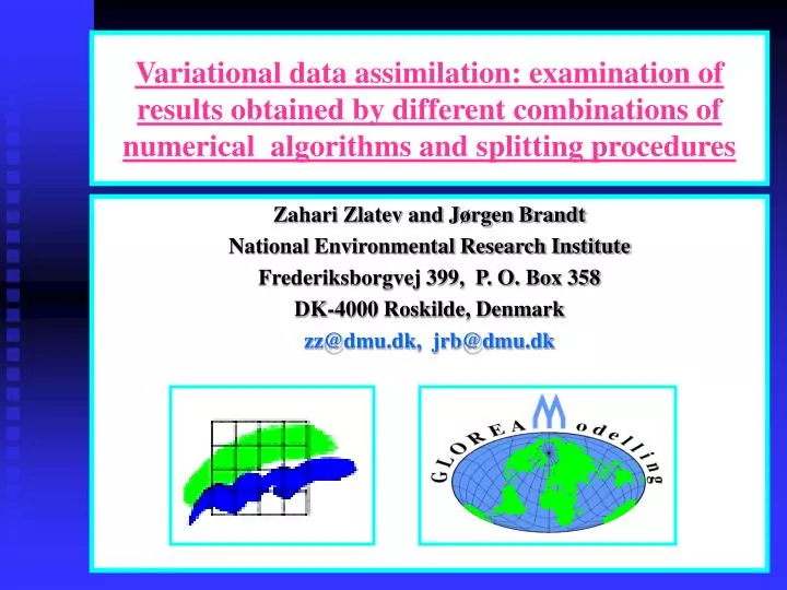
Variational data assimilation: examination of results obtained by different combinations of numerical algorithms and splitting procedures. Zahari Zlatev and Jørgen Brandt National Environmental Research Institute Frederiksborgvej 399, P. O. Box 358 DK-4000 Roskilde, Denmark

E N D
Variational data assimilation: examination of results obtained by different combinations of numerical algorithms and splitting procedures Zahari Zlatev and Jørgen Brandt National Environmental Research Institute Frederiksborgvej 399, P. O. Box 358 DK-4000 Roskilde, Denmark zz@dmu.dk, jrb@dmu.dk
CONTENTS • Some basic ideas • Optimization issues: calculation of the gradient of the object function • Algorithmic representation of the variational data assimilation • Tools: optimization methods, numerical algorithms and splitting procedures • Performance of the combination of the tools • Some conclusions
BASIC IDEAS - 1 An attempt to adjust globally the results of the model to the complete set of available observations (Talagrand and Courtier, 1987) Consistency between the dynamics of the model and the final results of the assimilation. (Talagrand and Courtier, 1987)
BASIC IDEAS - 2 Assumption: the variational data assimilation is used to improve the initial values of the resolved problem Variational data assimilation can be used for several other purposes (as, for example, to improve the quality of the emission fields).
Calculation of the gradient Assume that five fields (i.e. N=5) of observations are available
Calculation of the gradient Finishing the forward-backward calculations
Adjoint equations 1. Linear operators 2. Non-linear operators
Algorithmic representation INITIALIZE SCALAR VARIABLES, VECTORS AND ARRAYS; SET THE GRADIENT TO ZERO DO ITERATIONS = 1, MAX_ITERATIONS DO LARGE_STEPS = 1, P_STEP DO FORWARD_STEPS = (LARGE_STEPS – 1)*P_LENGTH + 1, LARGE_STEPS*P_LENGTH Perform a forward step with themodel END DO FORWARD_STEPS DO BACKWARD_STEPS = LARGE_STEPS*P_LENGTH, 1, -1 Perform a backward step with the adjoint equation END DO BACKWARD_STEPS UPDATE THE GRADIENT; COMPUTE THE VALUE OF THE OBJECT FUNCTION END DO LARGE_STEPS COMPUTE AN APPROXIMATION OF PARAMETER RHO UPDATE THE INITIAL VALUE FIELD (NEW FIELD = OLD FIELD - RHO*GRADIENT) CHECK THE STOPPING CRITERIA; IF SATISFIED EXIT FROM LOOP DO ITERATIONS END DO ITERATIONS PERFORM OUTPUT OPERATIONS AND STOP THE COMPUTATIONS
Applying splitting procedures Model Adjoint equation Model splitting Adjoint splitting
Computational tools A data assimilation code can be considered as a combination of three kinds of computational tools: • optimization methods, • numerical algorithms and • splitting procedures. It is important to understand that the choice of one of the tools is not independent of the choice of the others and the choice depends also on what is wanted in the particular study. Finding the optimal (or even only a good) combination of computational tools is a great challenge.
Splitting versus numerical errors Order of the numerical method: p Order of the splitting procedure: q Order of the combined methods: r = min(p,q) Synchronizing the choice of splitting procedures and numerical methods
Atmospheric chemical scheme • A chemical scheme containing 56 species has been used in the experiment • Species SO2, SO4, O3, NO, NO3, HNO3 PAN, NH3, NH4, OH and many hydrocarbons • Mathematical description: dc/dt = f(t,c) • Properties: • stiff • badly scaled • the solution varies in very wide range
Treatment of the chemical scheme • Six numerical methods • Backward Euler • Implicit Mid-point Rule • Two-stage Runge-Kutta • Three-stage Runge-Kutta • Two-stage Rosenbrock • Trapezoidal Rule • Five splittings • No splitting • Sequential splitting • Symmetric Splitting • Weighted sequential splitting • Weighted symmetric splitting
Some conclusions from the runs • The Backward Euler method is very robust for such problems, but might be expensive because its order of accuracy is only one. • The Implicit Mid-point Rule, the Trapezoidal Rule and the Three-stage Runge-Kutta method have difficulties. • The Two-stage Runge-Kutta Method and the Two-stage Rosenbrock Method are robust, but perform as first-order methods in spite of the fact that their actual order is two. • Major conclusion: It is not sufficient to have numerical methods of high order, it is also necessary to select methods with good stability properties (L-stability is actually needed).
Need for good stability properties Euler Mid-point Time-steps Error Rate Error Rate 144 9.0E-2 - 1.6E-2 - 288 4.5E-2 2.0 6.1E-3 2.6 576 2.3E-2 2.0 2.0E-3 3.0 1152 1.1E-2 2.0 6.2E-4 3.3 2304 5.6E-3 2.0 1.7E-4 3.6 4608 2.8E-3 2.0 4.4E-5 3.8 • Assimilation window: 6:00 - 12:00, observations at the end of every hour • Random perturbations of 25% are introduced in the ozone concentrations. • Data assimilation was applied using “exact” solutions as observations. • After the data assimilation procedure a forward run with the improved solution was performed on the interval from 6:00 to 12:00
Need for good stability properties-cont. Euler Mid-point Time-steps Error Rate Error Rate 1008 2.3E-1 - 3.2E-1 - 2016 1.1E-1 2.0 4.5E-2 6.5 4032 5.5E-2 2.0 8.8E-3 5.7 8064 2.7E-2 2.0 1.9E-2 0.5 16128 1.4E-2 2.0 2.2E-2 0.9 32256 6.8E-3 2.0 2.0E-2 1.4 • Assimilation window: 6:00 - 12:00, observations at the end of every hour • Random perturbations of 25% are introduced in the ozone concentrations. • Data assimilation was applied using “exact” solutions as observations. • After the data assimilation procedure a forward run with the improved solution was performed on the interval from 6:00 to 48:00
General conclusions • When will the variational data assimilation not work? • the discretization of the model is crude • the number of observations is very small (???) • When will the variational data assimilation work well? • there are sufficiently many observations • interpolation rules (or other similar devices) are used • the number of time-points at which observations are available is perhaps not very important • How to continue this research? • two-dimensional and three dimensional problems • more about the effect of splitting on data assimilation • order of accuracy of the data assimilation routines • interplay between ensembles and data assimilation