Download

1 / 49
490 likes | 625 Vues
“Erosion Research in Iowa”. Thanos N. Papanicolaou IIHR-Hydroscience and Engineering, University of Iowa. The Clear Creek Observatory, IA. The Clear Creek Observatory, IA. The Clear Creek Watershed coordinates. Testbed(s): nested watersheds in the Upper Mississippi River Basin.

E N D
“Erosion Research in Iowa” Thanos N. Papanicolaou IIHR-Hydroscience and Engineering, University of Iowa
The Clear Creek Watershed coordinates Testbed(s): nested watersheds in the Upper Mississippi River Basin
After Papanicolaou (2006), Geomorphology The Clear Creek Observatory, IA
The Clear Creek Observatory, IA Land-use Fingerprinting
The Clear Creek Observatory, IA f (biogeochemical processes) f ( factors ) δ15N δ13C C/N = = Using a Finnigan MAT Delta Plus isotope ratio mass spectrometer (IRMS)
The Clear Creek Observatory, IA δ15N= 4‰ δ15N= 2‰ Decomposition, mechanical breaking down of OM During decomposition, particles decrease in size. Also, the light N-14 atoms are incorporated into plant roots and thus the net change in δ15N is an increase relative to initial conditions. This is particularly important for soil-erosion considerations because particle size is a governing parameter.
Conclusions for Erosion studies: • The δ15N for monoculture wheat (C3) land-use reflects size distribution (after Fox and Papanicolaou JAWRA, 2007)
WEPP Model Calibration/verification • A hotspot model for NRCS people
Watershed Soil Characterization • 30% clay, 65% silt and ~ 5% sand. If clay is 20-40%, no stable aggregates formed, thus higher erosion. • pH range=6.0-7.0, range in which particles are most susceptible to erosion due to F to F contacts between clay particles • Cation Exchange Capacity were higher in cultivated soils i.e., corn = 25.7 cmol/kg and soybean = 35.1 cmol/kg than uncultivated soils.
Watershed Soil Characterization • Sodium adsorption ratio (SAR) was low for all soils which means higher erosion rate. • Mineralogy of clay – Majority Smectite, Vermiculite (and a small portion Kaolinite and Illite) have more water retention, hence lower shear required for soil erosion • Analyzed soil biogeochemical characteristics indicate that the catchment soil is highly erodible.
Results • Beginning with the 25 years simulation, equilibrium conditions for both water discharge and sediment discharge is reached
Results • The estimated avg. annual water discharge at the outlet is 5,775,717 m3/yr, sediment discharge is 26,335 ton/yr, and sediment delivery ratio is 0.183
Sample tray detail Bank sediment placed in sample tray detail Figure 6. A laboratory flume equipped with a sediment box sampler for testing critical erosional strength. Top to the right a bank sediment sample placed in the box sampler for testing its critical erosional strength.
ONE DIMENSIONAL HYDRODYNAMIC/SEDIMENT TRANSPORT MODEL TO SIMULATE RILL EROSION PROCESSES
Importance of Rills Sketch of upland erosional processes
Geomorphologic Features • Headcuts • Plunge pools • Steps: areas of locally flat and steep slopes • Rough, uneven bed profiles • Varying cross-sectional geometries (constrictions and expansions) • The process of rill evolution involves a feedback loop between erosion, hydraulics and bedform.
Geomorphologic Features Example of a step pool sequence often observed in rills
Rill Erosion • Rill erosion is a function of the capacity of the flow to detach sediment in relation to the capacity of the soil to resist detachment. • Depth-averaged velocity, discharge, and bed shear stress are used to express the capacity of the flow. • Rill sediment material is comprised of fines (clay, sand, silt, and organic material) • This material can exist as either fine suspended sediment or as aggregates of many particles that move as bedload (Gilley et al., 1990).
Primary Objectives and Goals The objective of this research is to develop a numerical model that removes some of the limitations of the existing models and accounts for the complex interaction of flow, geomorphology and sediment transport. The model proposed here is limited to 1-D flows and consists of a hydrodynamic and sediment transport component which are solved simultaneously.
Model Description: Hydrodynamic Component • 3ST1D (Steep Stream Sediment Transport 1-D) was previously developed for steep gravel bed streams. • It employs the TVD-MacCormack Scheme. • The Scheme solves the unsteady form of the St.Venant equations.
1 – D St. Venant Equations A = flow cross-sectional area Q = flow rate g = gravitational acceleration I1 = Hydrostatic Pressure force Term I2 = Forces exerted by channel wall contractions or expansions S0 = Bed Slop Sf = Friction slope = Momentum Coefficient
Conservative Form The conservative form of the equation guarantees correct jump intensities and celerities of surface waves (Lax and Wendroff, 1960).
TVD-MacCormack Scheme • Used to solve the 1-D St. Venant equations • Shock Capturing • Is a two step predictor-corrector scheme • Second order accurate and capable of rendering the solution ocsillation free (MacCormack, 1969)
Predictor Step Δt = time step Δx = cell size i = computational point j = time level n = Manning’s Roughness R = hydraulic radius
Corrector Step The corrector step uses the values of U and H from the predictor step
Results: Rill Bed (200 cells) Profiles Max error in water surface: Pools = 22% Step = 10%
Streamwise Distribution of Velocities (200 cells) Error in the predicted velocity values exceed 40% in the pools
Flow Continuity (200 Cells) Max Error in flow continuity 9%
Future Work • Incorporation of a channel dynamic model into WEPP for modeling flow and sediment in ditches and channels • Enhancement of the soil properties databases • Tracers for sediment provenance • There is still a need to define spatial variability of infiltration and runoff along a hillslope using new research methodologies and techniques. • In the Midwest the role of fertilizers (e.g., ammonia, manure), pesticides and etc. needs to be identified • Roughness characterization