Download
1 / 30
300 likes | 463 Vues
Probability and Limit States. Introduction to Engineering Systems Lecture 6 (9/14/2009). Prof. Andrés Tovar. Announcements. should be (1.25, 27). Print out Learning Center documents, read them, and bring them to Learning Center There’s a typo in HW2. Note on polyfit. x = 0:.2:1;

E N D
Probability and Limit States Introduction to Engineering Systems Lecture 6 (9/14/2009) Prof. Andrés Tovar
Announcements should be (1.25, 27) Print out Learning Center documents, read them, and bring them to Learning Center There’s a typo in HW2 Betting on a Design
Note on polyfit x = 0:.2:1; y_exp = [1.4 1.1 3.3 2.4 3.8 3.0]; c = polyfit(x, y_exp, 1); m = c(1); % slope b = c(2); % intercept y_fit = m*x + b; plot(x, y_exp, 'o') % plot experimental data hold on plot(x, y_fit, 'r') % plot best-fit line hold off • Note that polyfit only finds coefficients of line (slope and intercept). It does not plot the line. • need to add plot command to do this Betting on a Design
From last class • Basis function determines the empirical model. • Statistic is a numerical value that characterizes a dataset. • Mean or average (see also median and mode) • Standard deviation • Coefficient of variation • Uncertainty can be epistemic or aleatory. • Error can be systematic or random. Betting on a Design
Firing at a Target • = 17.2 m • = 1.4 m Adjust the pullback distance X of the slingshot to hit a target at a distance D downrange. How likely is it that a softball launched with a pullback of 1 m will land within 1 m of 17 m? Betting on a Design
Where to Aim the Slingshot? win $1 lose $5 • Suppose that you are required to take the following bet: • You will be paid $1 to launch a ball to less than 18 m. • But you will be fined $5 for each launch shorter than 16 m • What target distance should you aim for to maximize your gain? • How would you solve it? • What would you do differently if the fine were increased to $50? Betting on a Design
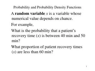
Probability number of successful outcomes estimated experimental probability of winning = total number of trials = probability of losing 1 – probability of winning • The relative frequency of possible outcomes • It is measured on a scale from 0 to 1 • Estimate probability by running an experiment with multiple trials • and counting number of favorable/unfavorable outcomes Betting on a Design
Coin toss • Suppose we run an experiment where we toss a coin 3 times H, H, T • What are the possible probabilities of the coin coming up “heads” that we could estimate from this experiment? 2/3 ≈ 0.6667 = 66.67% • What effect would using more trials have on our estimate? 1/2 = 0.5 = 50% Betting on a Design
More games 1/36 http://www.roulettebonuscode.com/ http://craps.gamble-world.com/ Theoretical probability of single events Betting on a Design
Example: Rolling a Die % simulation n = 100000; r = randi(6,1,n); wins = sum(r==1|r==6); losses = sum(r==2|r==3|r==4|r==5); simulated_gain = (5*wins - 2*losses)/n % theory p = 2; a = 5; q = 4; b = -2; theoretical_gain = (p*a + q*b)/(p + q) %#ok<*NOPTS> • Given a fair 6-sided die, what is your expected gain if: • you win $5 if you roll 1 or 6 • you lose $2 if you roll 2, 3, 4, or 5 • Should you take this bet? Betting on a Design
Expected Gain (or Loss) From a Bet expected gain • Huygens (again), 1656 • Given • p chances of winning a sum of money a • q chances of winning a sum of money b Betting on a Design
Estimating Probabilities for the Slingshot • For firing a slingshot with a pullback of 1 m. Estimate the probability that: • ball lands within 1 m of the target at 17 m. • ball lands short of this range (>18 m) • ball lands beyond this range (<16 m) Betting on a Design
Bin Counts Betting on a Design
Histogram Betting on a Design
Probabilities Betting on a Design
Theory of the Bell Curve: Normal Distribution flips from concave up to concave down 0.1% 2.1% 2.1% 0.1% 13.6% 13.6% 99.7% of distribution is between 3 99.9% of distribution is less than + 3 Betting on a Design
Experimental vs. theoretical distribution % distances of the softball D = [17.5 19.0 16.4 19.3 16.6 16.0 17.4 16.7 18.1 17.5 ... 15.1 14.2 17.4 15.7 17.8 19.3 18.5 15.7 17.9 17.0]; m = mean(D); % mean s = std(D); % standard deviation % experimental probability density y = 14:1:20; n = histc(D,y); bar(y+1/2,n/length(D),1); hold on xlabel('distanced (m)') ylabel('probabilityp(d)') % normal probability density itv = 0.0001; x = m-3*s:itv:m+3*s; p = 1/(s*sqrt(2*pi))*exp(-(x-m).^2/(2*s^2)); plot(x,p,'r.'); hold off p_theo=sum(p(x>=16 & x<=18))*itv p(16≤d≤18) = 0.55 (experimental) p(16≤d≤18) = 0.53 (normal distribution) Betting on a Design
The probabilities % distances of the softball D = [17.5 19.0 16.4 19.3 16.6 16.0 17.4 16.7 18.1 17.5 ... 15.1 14.2 17.4 15.7 17.8 19.3 18.5 15.7 17.9 17.0]; m = mean(D); % mean s = std(D); % standard deviation % plots itv = 0.0001; x = (m-3*s:itv:m+3*s); px = pdf('norm',m-3*s:itv:m+3*s,m,s); % probability density function figure(1); plot(x,px,'r.') % cumulative distribution function pxc = cdf('norm',m-3*s:itv:m+3*s,m,s); figure(2); plot(x,pxc,'b.') % results px16 = cdf('norm',16,m,s) % x<=16 pxm = cdf('norm',16:18,m,s); px17 = pxm(3)-pxm(1) % 16<x<=18 px18 = 1-cdf('norm',18,m,s) % x>18 Betting on a Design
Should we take the bet? p= 0.5280, a = 1 q = 0.2016, b = -5 Betting on a Design
DESIGN STAGE CONSTRUCTION & VERIFICATION Investigate Designs using Model Construct Design Optimize Design Experimentally Verify Behavior Predict Behavior Where we are in the tower design process MODEL DEVELOPMENT Gather Data Develop Model Verify Model Betting on a Design
Tower Bracing Betting on a Design
Design Considerations Betting on a Design
Limit States • Limit state: objective on the performance or behavior of a design • The consequences of failing to meet limit states can be very high • customer dissatisfaction (loss of business) • product recall • loss of property • loss of life • Terminology (“limit state design”) comes from structural engineering, but the concept cuts across all fields Betting on a Design
Limit States for Skyscraper Design Betting on a Design
Distribution of Tower Stiffness 0.07 N/mm Betting on a Design
Histogram of Tower Trial Stiffnesses m = 0.07 N/mm s = 0.02 N/mm Betting on a Design
How Good of a Fit for Tower Stiffnesses? = 0.07 = 0.02 • Pretty good fit! • We can use the normal distribution model to estimate probabilities Betting on a Design
Where to Aim for Tower Stiffness expensive pass limit state = 4.5N/19mm bracing cost fail cheap Betting on a Design
Confidence in Meeting Limit State Use probabilities from normal distribution to determine where to aim your design Betting on a Design
This week • The tower design problem • Factor of safety • Constraints • Efficiency • E = S/B • S = kbr/kubr: stiffness ratio • B = Lbr/Lubr: bracing ratio • Introduction to design optimization Betting on a Design