Download
1 / 59
610 likes | 917 Vues
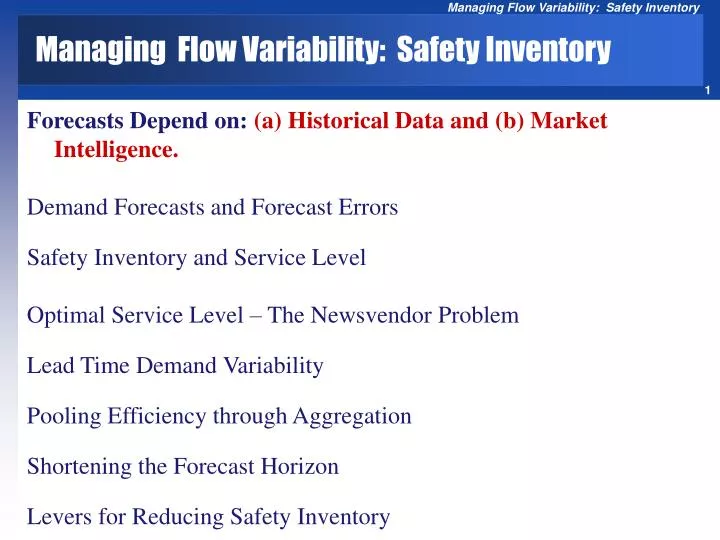
Managing Flow Variability: Safety Inventory. Forecasts Depend on: (a) Historical Data and (b) Market Intelligence. Demand Forecasts and Forecast Errors Safety Inventory and Service Level Optimal Service Level – The Newsvendor Problem Lead Time Demand Variability

E N D
Managing Flow Variability: Safety Inventory Forecasts Depend on: (a) Historical Data and (b) Market Intelligence. Demand Forecasts and Forecast Errors Safety Inventory and Service Level Optimal Service Level – The Newsvendor Problem Lead Time Demand Variability Pooling Efficiency through Aggregation Shortening the Forecast Horizon Levers for Reducing Safety Inventory
Four Characteristics of Forecasts • Forecasts are usually (always) inaccurate (wrong).Because of random noise. • Forecasts should be accompanied by a measure of forecast error.A measure of forecast error (standard deviation) quantifies the manager’s degree of confidence in the forecast. • Aggregate forecasts are more accurate than individual forecasts.Aggregate forecasts reduce the amount of variability – relative to the aggregate mean demand. StdDev of sum of two variables is less than sum of StdDev of the two variables. • Long-range forecasts are less accurate than short-range forecasts.Forecasts further into the future tends to be less accurate than those of more imminent events. As time passes, we get better information, and make better prediction.
Demand During Lead Time is Variable N(μ,σ) Demand of sand during lead time has an average of 50 tons. Standard deviation of demand during lead time is 5 tons Assuming that the management is willing to accept a risk no more that 5%.
Forecasts should be accompanied by a measure of forecast error Forecast and a Measure of Forecast Error
Demand During Lead Time Inventory Demand during LT Time Lead Time
Demand During Lead Time is Variable Inventory Time
Quantity A large demand during lead time Average demand during lead time ROP Safety stock Time LT Safety Stock Safety stock reduces risk of stockout during lead time
Quantity ROP Time LT Safety Stock
Re-Order Point: ROP Demand during lead time has Normal distribution. If we order when the inventory on hand is equal to the average demand during the lead time; then there is 50% chance that the demand during lead time is less than our inventory. However, there is also 50% chance that the demand during lead time is greater than our inventory, and we will be out of stock for a while. We usually do not like 50% probability of stock out We can accept some risk of being out of stock, but we usually like a risk of less than 50%.
Risk of a stockout Average demand Safety stock z-scale Safety Stock and ROP Service level Probability of no stockout ROP Quantity 0 z Each Normal variable x is associated with a standard Normal Variable z x is Normal (Average x , Standard Deviation x) z is Normal (0,1)
Service level Risk of a stockout Probability of no stockout ROP Quantity Average demand Safety stock 0 z z-scale z Values SL z value 0.9 1.28 0.95 1.65 0.99 2.33 • There is a table for z which tells us • Given anyprobability of not exceeding z. What is the value of z • Given anyvalue forz. What is the probability of not exceeding z
μand σ of Demand During Lead Time Demand of sand during lead time has an average of 50 tons. Standard deviation of demand during lead time is 5 tons. Assuming that the management is willing to accept a risk no more that 5%. Find the re-order point. What is the service level. Service level = 1-risk of stockout = 1-.05 = .95 Find the z value such that the probability of a standard normal variable being less than or equal to z is .95 Go to normal table, look inside the table. Find a probability close to .95. Read its z from the corresponding row and column.
Given a 95% SL 95% Probability The table will give you z Probability z Value using Table Page 319: Normal table 0.05 z Second digit after decimal Z = 1.65 Up to the first digit after decimal 1.6
F(z) z 0 The standard Normal Distribution F(z) F(z) = Prob( N(0,1) <z)
Service level Risk of a stockout Probability of no stockout ROP Quantity Average demand Safety stock 0 z z-scale Relationship between z and Normal Variable x z = (x-Average x)/(Standard Deviation of x) x = Average x +z (Standard Deviation of x) μ = Average x σ = Standard Deviation of x x = μ +z σ
Service level Risk of a stakeout Probability of no stockout ROP Quantity Average demand Safety stock 0 z z-scale Relationship between z and NormalVariable ROP LTD = Lead Time Demand ROP = Average LTD +z (Standard Deviation of LTD) ROP = LTD+zσLTD ROP = LTD + Isafety
Demand During Lead Time is Variable N(μ,σ) Demand of sand during lead time has an average of 50 tons. Standard deviation of demand during lead time is 5 tons Assuming that the management is willing to accept a risk no more that 5%. z = 1.65 Compute safety stock Isafety = zσLTD Isafety = 1.64 (5) = 8.2 ROP = LTD + Isafety ROP = 50 + 1.64(5) = 58.2
Service Level for a given ROP • SL= Prob (LTD ≤ ROP) • LTD is normally distributed LTD = N(LTD, sLTD). • ROP = LTD + zσLTD ROP = LTD + Isafety I safety = z sLTD • At GE Lighting’s Paris warehouse, LTD = 20,000, sLTD= 5,000 • The warehouse re-orders whenever ROP = 24,000 • I safety = ROP – LTD = 24,000 – 20,000 = 4,000 • I safety = z sLTD z = I safety / sLTD= 4,000 / 5,000 = 0.8 • SL= Prob (Z ≤ 0.8) from Appendix II SL= 0.7881
μ and σ of demand per period and fixed LT Demand of sand has an average of 50 tons per week. Standard deviation of the weekly demand is 3 tons. Lead time is 2 weeks. Assuming that the management is willing to accept a risk no more that 10%. Compute the Reorder Point
μ and σof demand per period and fixed LT R: demand rate perperiod(a random variable) R: Average demand rate perperiod σR:Standard deviation of the demand rate perperiod L: Lead time (a constant number of periods) LTD: demand during the lead time (a random variable) LTD: Average demand during the lead time σLTD:Standard deviation of the demand during lead time
μ and σ ofdemand per period and fixed LT A random variable R:N(R, σR) repeats itself L times during the lead time. The summation of these L random variables R, is a random variable LTD If we have a random variable LTD which is equal to summation of L random variables R LTD = R1+R2+R3+…….+RL Then there is a relationship between mean and standard deviation of the two random variables
μ and σ of demand per period and fixed LT Demand of sand has an average of 50 tons per week. Standard deviation of the weekly demand is 3 tons. Lead time is 2 weeks. Assuming that the management is willing to accept a risk no more that 10%. z = 1.28, R = 50, σR = 3, L = 2 Isafety = zσLTD = 1.28(4.24) = 5.43 ROP= 100 + 5.43
Lead Time Variable, Demand fixed Demand of sand is fixed and is 50 tons per week. The average lead time is 2 weeks. Standard deviation of lead time is 0.5 week. Assuming that the management is willing to accept a risk no more that 10%. Compute ROP and Isafety.
RL R L μ and σ oflead time and fixed Demand per period L: lead time (a random variable) L: Average lead time σL:Standard deviation of the lead time R: Demand per period (a constant value) LTD: demand during the lead time (a random variable) LTD: Average demand during the lead time σLTD:Standard deviation of the demand during lead time
RL R L μ and σ of demand per period and fixed LT A random variable L:N(L, σL) is multipliedby a constant R and generates the random variable LTD. If we have a random variable LTD which is equal to a constant Rtimes a random variables L LTD = RL Then there is a relationship between mean and standard deviation of the two random variables
R + R + R + R + R RL R R R R R R L L Variable R fixed L…………….Variable L fixed R
Lead Time Variable, Demand fixed Demand of sand is fixed and is 50 tons per week. The average lead time is 2 weeks. Standard deviation of lead time is 0.5 week. Assuming that the management is willing to accept a risk no more that 10%. Compute ROP and Isafety. z = 1.28, L = 2 weeks, σL = 0.5 week, R = 50 per week Isafety = zσLTD = 1.28(25) = 32 ROP= 100 + 32
Both Demand and Lead Time are Variable R: demand rate per period R: Average demand rate σR:Standard deviation of demand L: lead time L: Average lead time σL:Standard deviation of the lead time LTD: demand during the lead time (a random variable) LTD: Average demand during the lead time σLTD:Standard deviation of the demand during lead time
Optimal Service Level: The Newsvendor Problem How do we choose what level of service a firm should offer? Cost of Holding Extra Inventory Improved Service Optimal Service Level under uncertainty The Newsvendor Problem The decision maker balances the expected costs of ordering too much with the expected costs of ordering too little to determine the optimal order quantity.
Optimal Service Level: The Newsvendor Problem Cost =1800, Sales Price = 2500, Salvage Price = 1700 Underage Cost = 2500-1800 = 700, Overage Cost = 1800-1700 = 100 What is probability of demand to be equal to 130? What is probability of demand to be less than or equal to 140? What is probability of demand to be greater than 140? What is probability of demand to be equal to 133?
Optimal Service Level: The Newsvendor Problem What is probability of demand to be equal to 116? What is probability of demand to be less than or equal to 160? What is probability of demand to be greater than 116? What is probability of demand to be equal to 13.3?
Optimal Service Level: The Newsvendor Problem What is probability of demand to be equal to 130? What is probability of demand to be less than or equal to 140? What is probability of demand to be greater than 140? What is probability of demand to be equal to 133?
Compute the Average Demand Average Demand = +100×0.02 +110×0.05+120×0.08 +130×0.09+140×0.11 +150×0.16 +160×0.20 +170×0.15 +180×0.08 +190×0.05+200×0.01 Average Demand = 151.6 How many units should I have to sell 151.6 units (on average)? How many units do I sell (on average) if I have 100 units?
Suppose I have ordered 140 Unities. On average, how many of them are sold? In other words, what is the expected value of the number of sold units? When I can sell all 140 units? I can sell all 140 units if R≥ 140 Prob(R≥ 140) = 0.76 The the expected number of units sold –for this part- is (0.76)(140) = 106.4 Also, there is 0.02 probability that I sell 100 units 2 units Also, there is 0.05 probability that I sell 110 units5.5 Also, there is 0.08 probability that I sell 120 units 9.6 Also, there is 0.09 probability that I sell 130 units 11.7 106.4 + 2 + 5.5 + 9.6 + 11.7 = 135.2
Suppose I have ordered 140 Unities. On average, how many of them are salvaged? In other words, what is the expected value of the number of sold units? 0.02 probability that I sell 100 units. In that case 40 units are salvaged 0.02(40) = .8 0.05 probability to sell 110 30 salvage 0.05(30)= 1.5 0.08 probability to sell 120 30 salvage 0.08(20) = 1.6 0.09 probability to sell 130 30 salvage 0.09(10) =0.9 0.8 + 1.5 + 1.6 + 0.9 = 4.8 Total number Solved 135.2 @ 700 = 94640 Total number Salvaged 4.8 @ -100 = -480 Expected Profit = 94640 – 480 = 94,160
Analytical Solution for the Optimal Service Level Net Marginal Benefit: Net Marginal Cost: MB = p – c MC = c - v MB = $2,500 - $1,800 = $700 MC = $1,800 - $1,700 = $100 Suppose I have ordered Q units. What is the expected cost of ordering one more units? What is the expected benefit of ordering one more units? If I have ordered one unit more than Q units, the probability of not selling that extra unit is if the demand is less than or equal to Q. Since we have P( R ≤ Q). The expected marginal cost =MC× P( R ≤ Q) If I have ordered one unit more than Q units, the probability of selling that extra unit is if the demand is greater than Q. We know that P(R>Q) = 1- P( R ≤ Q). The expected marginal benefit = MB× [1-Prob.( R ≤ Q)]
Prob(R≤ Q*) ≥ In acontinuous model: SL* = Prob(R ≤ Q*) = Analytical Solution for the Optimal Service Level As long as expected marginal cost is less than expected marginal profit we buy the next unit. We stop as soon as: Expected marginal cost ≥ Expected marginal profit MC×Prob(R ≤ Q*) ≥ MB× [1 – Prob(R ≤ Q*)] If we assume demand is normally distributed, What quantity corresponds to this service level ?
Probability Less than Upper Bound is 0.87493 0.4 0.35 0.3 0.25 Density 0.2 z = 1.15 0.15 0.1 0.05 0 -4 -3 -2 -1 0 1 2 3 4 Critical Value (z) Analytical Solution for the Optimal Service Level
Aggregate Forecast is More Accurate than Individual Forecasts
Physical Centralization • Physical Centralization: the firm consolidates all its warehouses in one location from which is can serve all customers. • Example: Two warehouses. Demand in the two ware houses are independent. • Both warehouses have the same distribution for their lead time demand. • LTD1: N(LTD, σLTD )LTD2: N(LTD, σLTD ) • Both warehouses have identical service levels • To provide desired SL, each location must carry Isafety = zσLTD • z is determined by the desired service level • The total safety inventory in the decentralized system is
Independent Lead time demands at two locations • Decrease in safety inventory by a factor of LTDC = LTD1 + LTD2 LTDC = LTD + LTD = 2 LTD Centralization reduced the safety inventory by a factor of 1/√2 • GE lighting operating 7 warehouses. A warehouse with average lead time demand of 20,000 units with a standard deviation of 5,000 units and a 95% service level needs to carry a safety inventory of • Isafety = 1.65×5000= 8250
independent Lead time demands at N locations Independent demand in N locations: Total safety inventory to provide a specific SL increases not by N but by √N • Centralization of N locations: If centralization of stocks reduces inventory, why doesn’t everybody do it? • Longer response time • Higher shipping cost • Less understanding of customer needs • Less understanding of cultural, linguistics, and regulatory barriers These disadvantages my reduce the demand.
Dependent Demand • Does centralization offer similar benefits when demands in multiple locations are correlated? • LTD1 and LTD2are statistically identically distributed but correlated with a correlation coefficient of ρ . No Correlation: ρ close to 0