Download
1 / 38
380 likes | 443 Vues
Fluctuations in ISM Thermal Pressures Measured from C I Observations. Edward B. Jenkins Princeton University Observatory. Fundamentals …. Most of the free carbon atoms in the ISM are singly ionized, but a small fraction of the ions have recombined into the neutral form.

E N D
Fluctuations in ISM Thermal Pressures Measured from C I Observations Edward B. Jenkins Princeton University Observatory
Fundamentals … • Most of the free carbon atoms in the ISM are singly ionized, but a small fraction of the ions have recombined into the neutral form. • The ground electronic state of C I is split into three fine-structure levels with small energy separations. • Our objective is to study the relative populations of these three levels, which are influenced by local conditions (density & temperature.
Fine-structure Levels in the Ground State of C I Upper Electronic Levels Optical Pumping (by Starlight) Spontaneous Radiative Decays E/k = 62.4 K C I** 3P2 (E = 43.4 cm-1, g = 5) Collisionally Induced Transitions E/k = 23.6 K C I* 3P1 (E = 16.4 cm-1, g = 3) C I 3P0 (E = 0 cm-1, g = 1)
C I Absorption Features in the UV Spectrum of λ Cep Recorded at a Resolution of 1.5 km s-1 by STIS on HST From Jenkins & Tripp (2001: ApJS, 137, 297)
λ Cep C I Column density per unit velocity [1013 cm-2 (km s-1)-1] C I* C I** Velocity (km s-1)
Most Useful Way to Express Fine-structure Population Ratios • n(C I)total = n(C I) + n(C I*) + n(C I**) • f1 n(C I*)/n(C I)total • f2 n(C I**)/n(C I)total f2 Then consider the plot: Collision partners at a given density and temperature are expected to yield specific values of f1 and f2 f1
Collisional Excitation by Neutral H T = 100 K n(H) = 105 cm-3 n(H) = 104 cm-3 n(H) = 1000 cm-3 n(H) = 100 cm-3 n(H) = 10 cm-3
Collisional Excitation by Neutral H Plus Optical Pumping by the Average Galactic Starlight Field n(H) = 104 cm-3 n(H) = 1000 cm-3 n(H) = 100 cm-3 n(H) = 10 cm-3
Collisional Excitation by Neutral H Plus Optical Pumping by 10X the Average Galactic Starlight Field n(H) = 104 cm-3 n(H) = 1000 cm-3 n(H) = 100 cm-3 n(H) = 10 cm-3
Tracks for Different Temperatures T = 240 K T = 120 K n(H) = 100 cm-3 T = 60 K T = 30 K
Tracks for Different Temperatures T = 240 K T = 120 K p/k = 104 cm-3 K T = 60 K T = 30 K
A Theorem on how to deal with superpositions Cloud 2 Cloud 1
C I-weighted “Center of Mass” gives Composite f1,f2 A Theorem on how to deal with superpositions
Results • Original observations reported by Jenkins & Tripp (2001) included 21 stars. • We have now expanded this survey to about 100 stars by downloading from the MAST archive all suitable STIS observations that used the highest resolution echelle spectrograph (E140H). • The archival results have somewhat lower velocity resolution because the standard entrance aperture was usually used (instead of the extremely narrow slit chosen for the Jenkins & Tripp survey).
H II reg. T = 160K T = 80K T = 40K T = 20K Composite over all velocities and stars: f1 = 0.217, f2 = 0.073
H II reg. T = 160K T = 80K T = 40K T = 20K Note: HISA-land is down here
λ Cep Kinematics VDifferential Galactic Rotation VLSR C I Target Column density per unit velocity [1013 cm-2 (km s-1)-1] Sun C I* C I** Velocity (km s-1) (heliocentric) Positive Velocities Allowed Velocities Negative Velocities
H II reg. T = 160K T = 80K T = 40K T = 20K Allowed Velocities Composite f1 = 0.203, f2 = 0.063
H II reg. T = 160K T = 80K T = 40K T = 20K Positive Velocities Negative Velocities Composite f1 = 0.231, f2 = 0.082 for both velocity intervals
Barytropic index eff = 0.72 (Wolfire, Hollenbach, McKee, Tielens & Bakes 1995, ApJ 443, 152)
Log-normal Distribution of Mass vs. Density Relative Mass Fraction n(H I) (cm-3)
H I C I Log-normal distribution of H I mass fraction vs. n(H), with γeff = 5/3 Observed composite f1, f2
Observed composite f1, f2 H I C I Log-normal distribution of H I mass fraction vs. n(H), with γeff = 5/3
Observed composite f1, f2 H I C I Log-normal distribution of H I mass fraction vs. n(H), with γeff = 5/3
Observed composite f1, f2 H I C I Log-normal distribution of H I mass fraction vs. n(H), with γeff = 5/3
Observed composite f1, f2 H I C I Log-normal distribution of H I mass fraction vs. n(H), with γeff = 5/3
Observed composite f1, f2 H I C I Log-normal distribution of H I mass fraction vs. n(H), with γeff = 5/3
Model for a random mixture of high and low pressure gas Obs. Obs.
Pressure Distribution Function Note: The width of this peak is a lower limit, since the observations at each velocity probably exhibit some averaging of pressure extremes along the straight portion of the f1-f2 curve. H I mass fraction Relative Mass Fraction The width and central pressure of this peak are not well known, but the height of the peak is well determined. p/k (cm-3 K)
Pressure Distribution Function H I mass fraction C I mass fraction Relative Mass Fraction p/k (cm-3 K)
Could this component arise simply from the action of radiation or mass loss from the target stars (or their associations) either of which could compress the gas? Probably not: recall that negative velocity material behaved in much the same way as positive velocity material Blue = neg. vel. Red = pos. vel. A Question to Consider About the High Pressure Component Except for some gas parcels that have only high pressures
HS0624+6907 Galactic Coordinates: l = 145.7°, b = +23.4° Nearest O- or B-type star to the line of sight: 43 Cam (V = 5.14, spectral type: B7IV), about 2° away
Implications on the Existence of Small Neutral Stuctures Tcool = 2,500 yr Rapid Compression Tcool = 15,000 yr (for T = 60 K) Relative Mass Fraction p/k (cm-3 K)
Implications on the Existence of Small Neutral Stuctures • High pressure component mass fraction is low (~10-3), relative to most of the gas. • It has n(H I) ~ 103−104 cm-3 and T ≥ 100 K. • Tcool ≤ 2500 yr, which implies a typical dimension of only 0.00025 pc (i.e., 50 AU), or less, if crossing-time velocities are of order 10 km s-1 and the compression is nearly adiabatic.