Download

1 / 22
220 likes | 300 Vues
Surface Pressures from Space. R. A. Brown 2005 AGU. The Satellite + PBL Model calculation of surface pressure.

E N D
Surface Pressures from Space R. A. Brown 2005 AGU
The Satellite + PBL Model calculation of surface pressure • The microwave scatterometers, radiometers, SARs and altimeters have now provided nearly three decades of inferred surface winds over the oceans. These can all be converted to excellent surface pressure fields. • Often these products are revolutionary, changing the way we view the world. R. A. Brown 2005 AGU
The PBL Model (surface winds to pressures} R. A. Brown 2005 AGU
State of The analytic solution for a PBL fV + K Uzz - pz / = 0 fU - K Vzz + pz / = 0 The solution, U (f, K,p ) was found by Ekman in 1904. Unfortunately, this was almost never observed. fV + K Uzz - pz/ = 0 fU - K Vzz + pz/ = A(v2w2) Solution, U (f, K,p ) found in 1970. OLE are part of solution for 80% of observed conditions (near-neutral to convective). Unfortunately, this scale was difficult to observe. The complete nonlinear solution for OLE exists, including the 8th order instability solution, effects of variable roughness, stratification and baroclinicity, 1996. Integrated into MM5, NCEP (2005) R. A. Brown 2005 AGU
SLP from Surface Winds • UW PBL similarity model joins two layers: The nonlinear Ekman solution to the log layer solution. Use the “inverse” PBL model to estimate from satellite . Use vector math to get non-divergent field UG. Use Least-Square optimization to find best fit SLP to swaths: G (UG) = P(U10) → P(U10) There is extensive verification from ERS-1/2, NSCAT, QuikSCAT R. A. Brown 2005 AGU
The nonlinear solution applied to satellite surface winds yields accurate surface pressure fields. These data show: * The agreement between satellite and ECMWF pressure fields indicate that both the Scatterometer winds and the nonlinear PBL model (VG/U10) are accurate within 2 m/s. * A 3-month, zonally averaged offset angle <VG, U10> of 19° suggests that the mean marine PBL state is near neutral (the angle predicted by the nonlinear PBL model). * Swath deviation angle observations can be used to infer thermal wind and stratification. * Higher winds are obtained from pressure gradients and used as surface truth (rather than GCM or buoy winds). * VG (pressure gradients) rather than U10 could be used to initialize GCMs R. A. Brown 2005 AGU R. A. Brown 2005 EGU
The nonlinear PBL solution applied to satellite surface winds provides sufficient accuracy to determine surface pressure fields from satellite data alone. Patoux, J. and R.A. Brown, 2002: A Scheme for Improving Scatterometer Surface Wind Fields, J. Geophys. Res., 106, No. 20, pg 23,985-23,994 R. A. Brown 2005 AGU
R. A. Brown 2005 AGU R. A. Brown 2004 EGU
Dashed: ECMWF Solid: UW-Quikscat The UW PBL Model is now global R. A. Brown 2005 AGU
Surface Pressures QuikScat analysis ECMWF analysis J. Patoux & R. A. Brown
To get smooth synoptic wind fields from a scatterometer Raw scatterometer winds JPL Project Local GCM nudge smoothed = Dirth (with ECMWF fields) UW Pressure field smoothed R. A. Brown 2005 AGU R. A. Brown 2005 EGU
Pressure Fields used in NCEP Forecast Analyses R. A. Brown 2005 AGU
a b 996 991 999 996 OPC Sfc Analysis and IR Satellite Image 10 Jan 2005 0600 UTC GFS Sfc Analysis 10 Jan 2005 0600 UTC c d 984 982 UWPBL 10 Jan 2005 0600 UTC QuikSCAT 10 Jan 2005 0709 UTC
GFS 08 Jul 2005 OPC 08 Jul 2005 1003 996 996 b a UWPBL 08 Jul 2005 QuikSCAT 08 Jul 2005 1001 992 c d
Some Conclusions R. A. Brown 2005 AGU
Surface pressures as surface ‘truth’ yield high wind predictions. This suggests that the global climatology surface wind record is too low by 10 – 20%. Brown, R.A., & Lixin Zeng, 2001: Comparison of Planetary Boundary Layer Model Winds with Dropwindsonde Observations in Tropical Cyclones, J. Applied Meteor., 40, 10, 1718-1723; Foster & Brown, 1994, On Large-scale PBL Modelling: Surface Wind and Latent Heat Flux Comparisons, The Global Atmos.-Ocean System, 2, 199-219. R. A. Brown 2005 AGU
There is evidence from the satellite data that the secondary flow characteristics of the nonlinear PBL solution (Rolls or Coherent Structures) are present more often than not over the world’s oceans. This contributes to basic understanding of PBL modelling and air-sea fluxes. Brown, R.A., 2002: Scaling Effects in Remote Sensing Applications and the Case of Organized Large Eddies, Canadian Jn. Remote Sensing, 28, 340-345; Levy G., 2001, Boundary Layer RollStatistics from SAR. Geophysical Research Letters. 28(10),1993-1995. R. A. Brown 2005 AGU
The dynamics of the typical PBL revealed in remote sensing data indicate that K-theory in the PBL models is physically incorrect. This will mean revision of all GCM PBL models as resolution increases. Brown, R.A., 2001:On Satellite Scatterometer Model functions, J. Geophys. Res., Atmospheres, 105, n23, 29,195-29,205; Patoux, J. and R.A. Brown, 2001: Spectral Analysis of QuikSCAT Surface Winds and Two-Dimensional Turbulence, J. Geophys. Res., 106, D20, 23,995-24,005; Patoux, J. and R.A. Brown, 2002: A Gradient Wind Correction for Surface Pressure Fields Retrieved from Scatterometer Winds, Jn. Applied Meteor., Vol. 41, No. 2, pp 133-143; R.A. Brown & P. Mourad, 1990: A Model for K-Theory in a Multi-Scale Large Eddy Environment, AMS Preprint of Symposium on Turbulence and Diffusion, Riso, Denmark.On the Use of Exchange Coefficients and Organized Large Scale Eddies in Modeling Turbulent Flows. Bound. Layer Meteor., 20, 111-116, 1981. R. A. Brown 2005 AGU
Programs and Fields available onhttp://pbl.atmos.washington.eduQuestionsto rabrown, neal orjerome @atmos.washington.edu • Direct PBL model: PBL_LIB. (’75 -’05) An analytic solution for the PBL flow with rolls, U(z) = f( P, To , Ta , ) • The Inverse PBL model: Takes U10 field and calculates surface pressure field P (U10 , To , Ta , ) (1986 - 2005) • Pressure fields directly from the PMF: P (o) along all swaths (exclude 0 - 5° lat.?) (2001) (dropped in favor of I-PBL) • Global swath pressure fields for QuikScat swaths (with global I-PBL model) (2005) • Surface stress fields from PBL_LIB corrected for stratification effects along all swaths (2006) R. A. Brown 2005 AGU
Hazards of taking measurements in the Rolls Hodograph from convergentzone Hodograph from center zone 1-km The OLE winds Station A 3 U 2 - 5 km 2 The Mean Wind Z/ 1 Station B V Mean Flow Hodograph RABrown 2004
The solution for the PBL boundary layer (Brown, 1974, Brown and Liu, 1982), may be written U/VG = ei - e –z[e-iz + ieiz]sin +U2 where VG is the geostrophic wind vector, the angle between U10 and VG is [u*, HT, (Ta – Ts,)PBL] and the effect of the organized large eddies (OLE) in the PBL is represented by U2(u*, Ta – Ts, HT) This may be written: U/VG ={(u*), U2(u*), u*, zo(u*), VT(HT), (Ta – Ts), } OrU/VG= [u*, VT(HT), (Ta – Ts), , k, a]= {u*, HT, Ta – Ts}, for = 0.15, k= 0.4 and a = 1 In particular, Since: VG = (u*,HT, Ta – Ts) n(P, , f) HenceP= n [u*(o , k, a, ), HT, Ta – Ts, , f ] fn(o) R. A. Brown 2005 AGU
1980 – 2005: Using surface roughness as a lower boundary condition on the PBL, considerable information about the marine atmosphere and the PBL has been inferred from satellite data. The symbiotic relation between surface backscatter dataand the PBL model has been beneficial to both. • The PBL model has established superior ‘surface truth’ winds and pressures for the satellite model functions. • Satellite data have shown that the nonlinear PBL solution with Organized Large Eddies (OLE) is observed most of the time.