Download
1 / 45
450 likes | 585 Vues
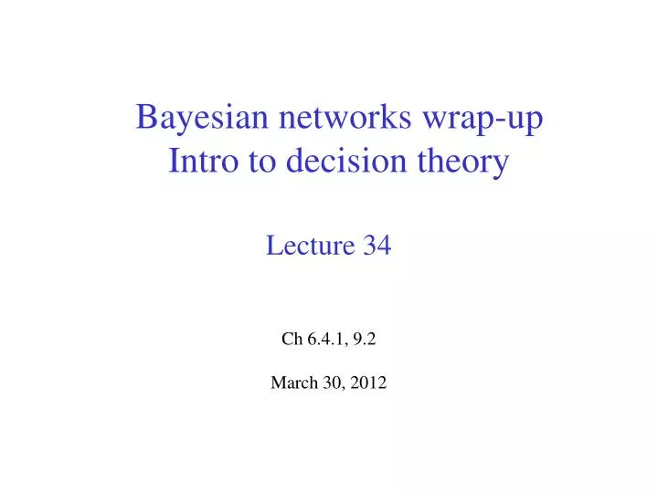
Bayesian networks wrap-up Intro to decision theory. Lecture 34 Ch 6.4.1, 9.2 March 30, 2012. Lecture Overview. Recap Lecture 33: Variable elimination (VE) for inference in Bnets VE example VE: pruning Decisions under Uncertainty Intro Utility (time permitting). Inference.

E N D
Bayesian networks wrap-up Intro to decision theory Lecture 34 Ch 6.4.1, 9.2 March 30, 2012
Lecture Overview • Recap Lecture 33: Variable elimination (VE) for inference in Bnets • VE example • VE: pruning • Decisions under Uncertainty • Intro • Utility (time permitting)
Inference • Y: subset of variables that is queried • E: subset of variables that are observed . E = e • Z1, …,Zkremaining variables in the JPD • We need to compute this numerator for each value of Y, yi • We need to marginalize over all the variables Z1,…Zk not involved in the query Def of conditional probability • To compute the denominator, marginalize over Y • - Same value for every P(Y=yi). Normalization constant ensuring that • All we need to compute is the numerator: joint probability of the query variable(s) • and the evidence! • Variable Elimination is an algorithm that efficiently performs this operation by • casting it as operations between factors - introduced next
Factors • A factor is a function from a tuple of random variables to the real numbers R • We write a factor on variables X1,… ,Xjas f(X1,… ,Xj) • A factor denotes one or more (possibly partial) distributions over the given tuple of variables, e.g., • P(X1, X2) is a factor f(X1, X2) • P(Z | X,Y) is a factor • f(Z,X,Y) • P(Z=f|X,Y) is a factor f(X,Y) • Note: Factors do not have to sum to one Distribution Set of Distributions One for each combination of values for X and Y f(X, Y ) Z = f Set of partial Distributions
Operation 1: assigning a variable • We can make new factors out of an existing factor • Our first operation:we can assign some or all of the variables of a factor. • What is the result of assigning X= t ? f(X=t,Y,Z) =f(X, Y, Z)X = t Factor of Y,Z
Operation 2: Summing out a variable • Our second operation on factors: we can marginalize out (or sum out) a variable • Exactly as before. Only difference: factors don’t sum to 1 • Marginalizing out a variable X from a factor f(X1,… ,Xn) yields a new factor defined on {X1,… ,Xn } \ {X} (Bf3)(A,C)
Operation 3: multiplying factors The product of factor f1(A, B) and f2(B, C), where B is the variable in common, is the factor (f1× f2)(A, B, C) defined by: f1(A,B)× f2(B,C):
6. Normalize by dividing the resulting factor f(Y) by The variable elimination algorithm, The JPD of a Bayesian network is • Construct a factor for each conditional probability. • For each factor, assign the observed variables E to their observed values. • Given an elimination ordering, decompose sum of products • Sum out all variables Zinot involved in the query (one a time) • Multiply factors containing Zi • Then marginalize out Zifrom the product • Multiply the remaining factors (which only involve Y ) • We make a factor fi for each conditional probability • So we have To compute P(Y=yi| E = e) See the algorithm VE_BN in the P&M text, Section 6.4.1, Figure 6.8, p. 254.
Lecture Overview • Recap Lecture 33: Variable elimination (VE) for inference in Bnets • VE example • VE: pruning • Decisions under Uncertainty • Intro • Utility (time permitting)
Variable elimination example Compute P(G|H=h1). P(G,H) = A,B,C,D,E,F,IP(A,B,C,D,E,F,G,H,I) = = A,B,C,D,E,F,IP(A)P(B|A)P(C)P(D|B,C)P(E|C)P(F|D)P(G|F,E)P(H|G)P(I|G)
Step 1: Construct a factor for each cond. probability Compute P(G|H=h1). P(G,H) = A,B,C,D,E,F,IP(A)P(B|A)P(C)P(D|B,C)P(E|C)P(F|D)P(G|F,E)P(H|G)P(I|G) P(G,H) = A,B,C,D,E,F,If0(A) f1(B,A) f2(C) f3(D,B,C) f4(E,C) f5(F, D) f6(G,F,E) f7(H,G) f8(I,G) • f0(A) • f1(B,A) • f2(C) • f3(D,B,C) • f4(E,C) • f5(F, D) • f6(G,F,E) • f7(H,G) • f8(I,G)
Step 2: assign to observed variables their observed values. Compute P(G|H=h1). Previous state: P(G,H) = A,B,C,D,E,F,I f0(A) f1(B,A) f2(C) f3(D,B,C) f4(E,C) f5(F, D) f6(G,F,E) f7(H,G) f8(I,G) ObserveH : P(G,H=h1)=A,B,C,D,E,F,I f0(A) f1(B,A) f2(C) f3(D,B,C) f4(E,C) f5(F, D) f6(G,F,E) f9(G) f8(I,G) • f0(A) • f1(B,A) • f2(C) • f3(D,B,C) • f4(E,C) • f5(F, D) • f6(G,F,E) • f7(H,G) • f8(I,G) • f9(G) H=h1
Step 3: Decompose sum of products Compute P(G|H=h1). Previous state: P(G,H=h1) = A,B,C,D,E,F,If0(A) f1(B,A) f2(C) f3(D,B,C) f4(E,C) f5(F, D) f6(G,F,E)f9(G)f8(I,G) Elimination ordering A, C, E, I, B, D, F: P(G,H=h1) = f9(G) F D f5(F, D) B I f8(I,G)E f6(G,F,E)C f2(C) f3(D,B,C) f4(E,C) A f0(A) f1(B,A) • f0(A) • f1(B,A) • f2(C) • f3(D,B,C) • f4(E,C) • f5(F, D) • f6(G,F,E) • f7(H,G) • f8(I,G) • f9(G)
Step 4: sum out non query variables (one at a time) Compute P(G|H=h1). Elimination order: A,C,E,I,B,D,F Previous state: P(G,H=h1) = f9(G) F D f5(F, D) B I f8(I,G)E f6(G,F,E) C f2(C) f3(D,B,C) f4(E,C) A f0(A) f1(B,A) Eliminate A: perform product and sum out A in P(G,H=h1) = f9(G) F D f5(F, D) B f10(B) I f8(I,G)E f6(G,F,E) C f2(C) f3(D,B,C) f4(E,C) • f10(B) does not depend • on C, E, or I, so we can • push it outside of those • sums. • f9(G) • f0(A) • f1(B,A) • f2(C) • f3(D,B,C) • f4(E,C) • f5(F, D) • f6(G,F,E) • f7(H,G) • f8(I,G) • f10(B)
Step 4: sum out non query variables (one at a time) Compute P(G|H=h1). Elimination order: A,C,E,I,B,D,F Previous state: P(G,H=h1) = f9(G) F D f5(F, D) B f10(B)I f8(I,G)E f6(G,F,E) C f2(C) f3(D,B,C) f4(E,C) Eliminate C: perform product and sum out C in P(G,H=h1) = f9(G) F D f5(F, D) B f10(B)I f8(I,G)E f6(G,F,E)f11(B,D,E) • f9(G) • f0(A) • f1(B,A) • f2(C) • f3(D,B,C) • f4(E,C) • f5(F, D) • f6(G,F,E) • f7(H,G) • f8(I,G) • f10(B) • f11(B,D,E)
Step 4: sum out non query variables (one at a time) Compute P(G|H=h1). Elimination order: A,C,E,I,B,D,F Previous state: P(G,H=h1) = P(G,H=h1) = f9(G) F D f5(F, D) B f10(B)I f8(I,G)E f6(G,F,E)f11(B,D,E) Eliminate E: perform product and sum out E in P(G,H=h1) = P(G,H=h1) = f9(G) F D f5(F, D) B f10(B) f12(B,D,F,G) I f8(I,G) • f9(G) • f0(A) • f1(B,A) • f2(C) • f3(D,B,C) • f4(E,C) • f5(F, D) • f6(G,F,E) • f7(H,G) • f8(I,G) • f10(B) • f11(B,D,E) • f12(B,D,F,G)
Step 4: sum out non query variables (one at a time) Compute P(G|H=h1). Elimination order: A,C,E,I,B,D,F Previous state: P(G,H=h1) = P(G,H=h1) = f9(G) F D f5(F, D) B f10(B)f12(B,D,F,G) If8(I,G) Eliminate I: perform product and sum out I in P(G,H=h1) = P(G,H=h1) = f9(G) f13(G)F D f5(F, D) B f10(B)f12(B,D,F,G) • f9(G) • f0(A) • f1(B,A) • f2(C) • f3(D,B,C) • f4(E,C) • f5(F, D) • f6(G,F,E) • f7(H,G) • f8(I,G) • f10(B) • f11(B,D,E) • f12(B,D,F,G) • f13(G)
Step 4: sum out non query variables (one at a time) Compute P(G|H=h1). Elimination order: A,C,E,I,B,D,F Previous state: P(G,H=h1) = P(G,H=h1) = f9(G) f13(G)F D f5(F, D) B f10(B) f12(B,D,F,G) Eliminate B: perform product and sum out B in P(G,H=h1) = P(G,H=h1) = f9(G) f13(G)F D f5(F, D) f14(D,F,G) • f9(G) • f0(A) • f1(B,A) • f2(C) • f3(D,B,C) • f4(E,C) • f5(F, D) • f6(G,F,E) • f7(H,G) • f8(I,G) • f10(B) • f11(B,D,E) • f12(B,D,F,G) • f13(G) • f14(D,F,G)
Step 4: sum out non query variables (one at a time) Compute P(G|H=h1). Elimination order: A,C,E,I,B,D,F Previous state: P(G,H=h1) = P(G,H=h1) = f9(G) f13(G)F D f5(F, D) f14(D,F,G) Eliminate D: perform product and sum out D in P(G,H=h1) = P(G,H=h1) = f9(G) f13(G)F f15(F,G) • f9(G) • f0(A) • f1(B,A) • f2(C) • f3(D,B,C) • f4(E,C) • f5(F, D) • f6(G,F,E) • f7(H,G) • f8(I,G) • f10(B) • f11(B,D,E) • f12(B,D,F,G) • f13(G) • f14(D,F,G) • f15(F,G)
Step 4: sum out non query variables (one at a time) Compute P(G|H=h1). Elimination order: A,C,E,I,B,D,F Previous state: P(G,H=h1) = P(G,H=h1) = f9(G) f13(G)F f15(F,G) Eliminate F: perform product and sum out F in f9(G) f13(G)f16(F,G) • f9(G) • f0(A) • f1(B,A) • f2(C) • f3(D,B,C) • f4(E,C) • f5(F, D) • f6(G,F,E) • f7(H,G) • f8(I,G) • f10(B) • f11(B,D,E) • f12(B,D,F,G) • f13(G) • f14(D,F,G) • f15(F,G) • f16(G)
Step 5: Multiply remaining factors Compute P(G|H=h1). Elimination order: A,C,E,I,B,D,F Previous state: P(G,H=h1) = f9(G) f13(G)f16(G) Multiply remaining factors (all in G): P(G,H=h1) =f17(G) • f9(G) • f0(A) • f1(B,A) • f2(C) • f3(D,B,C) • f4(E,C) • f5(F, D) • f6(G,F,E) • f7(H,G) • f8(I,G) • f10(B) • f11(B,D,E) • f12(B,D,F,G) • f17(G) • f13(G) • f14(D,F,G) • f15(F,G) • f16(G)
Step 6: Normalize Compute P(G|H=h1). • f9(G) • f0(A) • f1(B,A) • f2(C) • f3(D,B,C) • f4(E,C) • f5(F, D) • f6(G,F,E) • f7(H,G) • f8(I,G) • f10(B) • f11(B,D,E) • f12(B,D,F,G) • f17(G) • f13(G) • f14(D,F,G) • f15(F,G) • f16(G)
Lecture Overview • Recap Lecture 33: Variable elimination (VE) for inference in Bnets • VE example • VE: pruning • Decisions under Uncertainty • Intro • Utility (time permitting)
Complexity of Variable Elimination (VE) • A factor over n binary variables has to store 2n numbers • The initial factors are typically quite small (variables typically only have few parents in Bayesian networks) • But variable elimination constructs larger factors by multiplying factors together • The complexity of VE is exponential in the maximum number of variables in any factor during its execution • This number is called the treewidth of a graph (along an ordering) • Elimination ordering influences treewidth • Finding the best ordering is NP complete • I.e., the ordering that generates the minimum treewidth • Heuristics work well in practice (e.g. least connected variables first) • Even with best ordering, inference is sometimes infeasible • In those cases, we need approximate inference. See CS422 & CS540
VE and conditional independence • So far, we haven’t use conditional independence! • Before running VE, we can prune all variables Z that are conditionally independent of the query Y given evidence E: Z ╨ Y | E • They cannot change the belief over Y given E! • Example: which variables can we prune for the query P(G=g| C=c1, F=f1, H=h1) ? A B D E
Variable elimination: pruning • We can also prune unobserved leaf nodes • Since they are unobserved and not predecessors of the query nodes, they cannot influence the posterior probability of the query nodes • Thus, if the query is • P(G=g| C=c1, F=f1, H=h1) • we only need to consider this • subnetwork Slide 26
One last trick • We can also prune unobserved leaf nodes • And we can do so recursively • E.g., which nodes can we prune if the query is P(A)? H I G All nodes other than A
VE in AISpace • To see how variable elimination works in the Aispace Applet • Select “Network options -> Query Models > verbose” • Compare what happens when you select “Prune Irrelevant variables” or not in the VE window that pops up when you query a node • Try different heuristics for elimination ordering
Learning Goals For VE • Variable elimination • Understating factors and their operations • Carry out variable elimination by using factors and the related operations • Use techniques to simplify variable elimination
Big picture: Reasoning Under Uncertainty Probability Theory Bayesian Networks & Variable Elimination Dynamic Bayesian Networks Hidden Markov Models & Filtering Monitoring(e.g. credit card fraud detection) Bioinformatics Motion Tracking,Missile Tracking, etc Natural Language Processing Diagnostic systems(e.g. medicine) Email spam filters
One Realistic BN: Liver DiagnosisSource: Onisko et al., 1999 ~60 nodes, max 4 parents per node
Realistic BNet: Student TracingSource: ConatiGertner and VanLehn 2002 • Andes Tutor for Physics captures student problem solving actions • Sends them as evidence to a Bnet that assesses student knowledge of relevant physics principles • Based on the network prediction, Andes provides interactive help to the student • Used routinely at the US Naval Academy as homework aid
Where are we? Representation • Environment Reasoning Technique Stochastic Deterministic Problem Type This concludes the module on answering queries in stochastic environments Arc Consistency Constraint Satisfaction Vars + Constraints Search Static Belief Nets Logics Variable Elimination Query Search Decision Nets Sequential STRIPS Variable Elimination Planning Search
What’s Next? Representation • Environment Reasoning Technique Stochastic Deterministic Problem Type Arc Consistency Now we will look at acting in stochastic environments Constraint Satisfaction Vars + Constraints Search Static Belief Nets Logics Variable Elimination Query Search Decision Nets Sequential STRIPS Variable Elimination Planning Search
Lecture Overview • Recap Lecture 33: Variable elimination (VE) for inference in Bnets • VE example • VE: pruning • Decisions under Uncertainty • Intro • Utility (time permitting)
Decisions Under Uncertainty: Intro • Earlier in the course, we focused on decision making in deterministic domains • Search/CSPs: single-stage decisions • Planning: sequential decisions • Now we face stochastic domains • so far we've considered how to represent and update beliefs • what if an agent has to make decisions (act) under uncertainty? • Making decisions under uncertainty is important • We represent the world probabilistically so we can use our beliefs as the basis for making decisions
Decisions Under Uncertainty: Intro • An agent's decision will depend on • What actions are available • What beliefs the agent has • Which goals the agent has • Differences between deterministic and stochastic setting • Obvious difference in representation: need to represent our uncertain beliefs • Actions will be pretty straightforward: represented as decision variables • Goals will be interesting: we'll move from all-or-nothing goals to a richer notion: • rating how happy the agent is in different situations. • Putting these together, we'll extend Bayesian Networks to make a new representation called Decision Networks
Delivery Robot Example • Robot needs to reach a certain room • Robot can go • the short way - faster but with more obstacles, thus more prone to accidents that can damage the robot • the long way - slower but less prone to accident • Which way to go? Is it more important for the robot to arrive fast, or to minimize the risk of damage? • The Robot can choose to wear pads to protect itself in case of accident, or not to wear them. Pads slow it down • Again, there is a tradeoff between reducing risk of damage and arriving fast • Possible outcomes • No pad, no accident • Pad, no accident • Pad, Accident • No pad, accident
Next • We’ll see how to represent and reason about situations of this nature using Decision Trees, as well as • Probability to measure the uncertainty in action outcome • Utility to measure agent’s preferences over the various outcomes • Combined in a measure of expected utility that can be used to identify the action with the best expected outcome • Best that an intelligent agent can do when it needs to act in a stochastic environment
Decision Tree for the Delivery Robot Example • Decision variable 1: the robot can choose to wear pads • Yes: protection against accidents, but extra weight • No: fast, but no protection • Decision variable 2: the robot can choose the way • Short way: quick, but higher chance of accident • Long way: safe, but slow • Random variable: is there an accident? Agent decides Chance decides
Delivery Robot Example • Decision variable 1: the robot can choose to wear pads • Yes: protection against accidents, but extra weight • No: fast, but no protection • Decision variable 2: the robot can choose the way • Short way: quick, but higher chance of accident • Long way: safe, but slow • Random variable: is there an accident? Agent decides Chance decides
Possible worlds and decision variables • A possible world specifies a value for each random variable and each decision variable • For each assignment of values to all decision variables • the probabilities of the worlds satisfying that assignment sum to 1. 0.2 0.8
Possible worlds and decision variables • A possible world specifies a value for each random variable and each decision variable • For each assignment of values to all decision variables • the probabilities of the worlds satisfying that assignment sum to 1. 0.2 0.8 0.01 0.99
Possible worlds and decision variables • A possible world specifies a value for each random variable and each decision variable • For each assignment of values to all decision variables • the probabilities of the worlds satisfying that assignment sum to 1. 0.2 0.8 0.01 0.99 0.2 0.8
Possible worlds and decision variables • A possible world specifies a value for each random variable and each decision variable • For each assignment of values to all decision variables • the probabilities of the worlds satisfying that assignment sum to 1. 0.2 0.8 0.01 0.99 0.2 0.8 0.01 0.99