Download
1 / 86
870 likes | 1.16k Vues
e. L. k. i. o. h. o. i. d. l. Likelihood, Bayesian and Decision Theory. Kenneth Yu. History. The likelihood principle was first introduced by R.A. Fisher in 1922. The law of likelihood was identified by Ian Hacking.

E N D
e L k i o h o i d l
Likelihood, Bayesian and Decision Theory Kenneth Yu
History • The likelihood principle was first introduced by R.A. Fisher in 1922. The law of likelihood was identified by Ian Hacking. • "Modern statisticians are familiar with the notion that any finite body of data contains only a limited amount of information on any point under examination; that this limit is set by the nature of the data themselves…the statistician's task, in fact, is limited to the extraction of the whole of the available information on any particular issue." R. A. Fisher
Likelihood Principle • All relevant data in is contained in the likelihood function L(θ | x) = P(X=x | θ) Law of Likelihood • The extent to which the evidence supports one parameter over another can be measured by taking their ratio • These two concepts allow us to utilize likelihood for inferences on θ.
Motivation and Applications • Likelihood (Especially MLE) is used in a range of statistical models such as structural equation modeling, confirmatory factor analysis, linear models, etc. to make inferences on the parameter in a function. Its importance came from a need to find the “best” parameter value subject to error. • This makes use of only the evidence and disregards the prior probability of the hypothesis. By making inferences on unknown parameters from our past observations, we are able to estimate the true Θ value for the population.
The Likelihood is a function of the form: L(Θ|X)Є{α P(X|Θ) : α > 0 } • This represents how “likely” Θ is if we have prior outcomes X. It is the same as the probability of X happening given parameter Θ • Likelihood functions are equivalent if they differ by constant α (They are proportional). The inferences on parameter Θ would be the same if based on equivalent functions.
Maximum Likelihood Method By Hanchao
Main topic include: • 1. Why use Maximum Likelihood Method? • 2. Likelihood Function • 3. Maximum Likelihood Estimators • 4. How to calculate MLE?
1. Why use Maximum Likelihood Method? Difference between: Method of Moments & Method of Maximum likelihood
Mostly, same! • However, Method of Maximum likelihood does yield “good” estimators: 1. an after-the-fact calculation 2. More versatile methods for fitting parametric statistical models to data 3. Suit for large data samples
2. Likelihood Function • Definition: Let , be the joint probability (or density) function of n random variables : with sample values The likelihood function of the sample is given by:
If are discrete iid random variable with probability function , then, the likelihood functionis given by
In the continuous case, if the density is then, the likelihood function is given by i.e. Let be iid random variables. Find the Likelihood function?
4. Procedure of one approach to find MLE • 1). Define the likelihood function, L(θ) • 2). Take the natural logarithm (ln) of L(θ) • 3). Differentiate ln L(θ) with respect to θ, and then equate the derivative to 0. • 4). Solve the parameter θ, and we will obtain • 5). Check whether it is a max or global max • Still confuse?
Ex1: Suppose are random samples from a Poisson distribution with parameter λ. Find MLE ? We have pmf: Hence, the likelihood function is:
Differentiating with respect to λ, results in: And let the result equals to zero: That is, Hence, the MLE of λ is:
Ex2: Let be .a) if μ is unknown and is known, find the MLE for μ.b) if is known and unknown, find the MLE for .c) if μ and are both unknown, find the MLE for . • Ans: Let , so the likelihood function is:
So after take the natural log we have: a). When is known, we only need to solve the unknown parameter μ:
b) When is known, so we only need to solve one parameter : • c) When both μ and θ unknown, we need to differentiate both parameters, and mostly follow the same steps by part a). and b).
Reality example: Sound localization Mic2 Mic1 MCU
Robust Sound LocalizationIEEE Transactions on Signal Processing, Vol. 53, No. 6, June 2005 Noise reverberations Sound Source
The ideality and reality Mic1 Mic2 The received signal in 1meter and angle 60 frequency 1kHz
Fourier Transform shows noise Amplitude Frequency (100Hz)
Algorithm: 1. Signal collection (Original signal samples in time domain) 2. Cross Correlation (received signals after DFT, in freq domain)
However, we have noise mixing within the signal, so the Weighting Cross Correlation algorithm become: • Where by Using ML method as “Weighting function ” to reduce the sensitive from noise & reverberations
Reference: The disadvantage of MLE • Complicated calculation (slow) -> it is almost the last approach to solve the problem • Approximated results (not exact) [1] Halupka, 2005,Robust sound localization in 0.18 um CMOS [2] S.Zucker, 2003, Cross-correlation and maximum-likelihood analysis: a new approach to combining cross-correlation fuctions [3]Tamhane Dunlop, “Statistics and Data Analysis: from Elementary to intermediate”, Chap 15. [4]Kandethody M. Ramachandran, Chris P. Tsokos, “Mathematical Statistics with Applications”, page 235-252.
Likelihood ratio test Ji Wang
Brief Introduction • The likelihood ratio test was firstly claimed by Neyman and E.pearson in 1928. This test method is widely used and always has some kind of optimality. • In statistics, a likelihood ratio test is used to compare the fit of two models, one of which is nested within the other. This often occurs when testing whether a simplifying assumption for a model is valid, as when two or more model parameters are assumed to be related.
Introduction about most powerful test To the hypothesis , we have two test functions and , If *, ,then we called is more powerful than . If there is a test function Y satisfying the * inequality to the every test function , then we called Y the uniformly most powerful test.
The advantage of likelihood ratio test comparing to the significance test • The significance testcan only deal with the hypothesis in specific interval just like: but can not handle the very commonly hypothesis : because we can not use the method of significance test to find the reject region.
Definition of likelihood ratio test statistic • are the random identical sampling from the family distribution of F={ }. For the test let We call is the likelihood ratio of the above mentioned hypothesis. Sometimes we also called it general likelihood ratio. # From the definition of the likelihood ratio test statistics, we can find if the value of is small, the null hypothesis is more probably to occur than the alternative hypothesis , so it is reasonable for us to reject null hypothesis. Thus, this test reject if
The definition of likelihood ratio test • We use as the test statistic of the test : and the rejection region is , the C satisfy the inequality Then this test is the likelihood ratio test of level. #If we do not know the distribution of under null hypothesis, it is very difficult for us to find the marginal value of LRT. However, if there is a statistic( )which is monotonous to the ,and we know its distribution under null hypothesis. Thus, we can make a significance test based on the .
The steps to make a likelihood ratio test • Step1 Find the likelihood ration function of the sample . • Step2 Find the , the test statistic or some other statistics which is monotonous to the . • Step3 Construct the reject region by using the type 1 error at the significance level of .
Example are the random samples having the pdf: Please derive the rejection region of the hypothesis in the level
Solution: ● Step1: the sample distribution is : and it is also the likelihood function, the parameter space is then we derived
● Step2 the likelihood ratio test statistics We can just used ,because it is monotonous to the ● Step3 Under the null hypothesis, , so the marginal value by calculating the That is to say is the likelihood ratio test statistics and the reject region is
Xiao Yu Wald Sequential Probability Ratio Test So far we assumed that the sample size is fixed in advance. What if it is not fixed? Abraham Wald(1902-1950) developed the sequential probability ratio test(SPRT) by applying the idea of likelihood ratio testing, which sample sequentially by taking observations one at a time.
Hypothesis: • If stop sampling and decide to not reject • If continue sampling • If stop sampling and decide to reject
SPRT for Bernoulli Parameter • A electrical parts manufacturer receives a large lot of fuses from a vendor. The lot is regarded as “satisfactory” if the fraction defective p is no more than 0.1, otherwise it is regarded as “unsatisfactory”.
Fisher Information score Cramer-Rao Lower Bound
Single-Parameter Bernoulli experiment • The Fisher information contained n independent Bernoulli trials may be calculated as follows. In the following, A represents the number of successes, B the number of failure. We can see it’s reciprocal of the variance of the number of successes in N Bernoulli trials. The more the variance, the less the Fisher information.
Large Sample Inferences Based on the MLE’s • An approximate large sample (1-alpha)-level confidence interval(CI) is given by Plug in the Fisher information of Bernoulli trials, we can see it’s consistent as we have learned.
Bayes' theorem Jaeheun kim Thomas Bayes (1702 –1761) -English mathematician and a Presbyterian minister born in London -a specific case of the theorem (Bayes'theorem), which was published after his death (Richard price)
Bayesian inference • Bayesian inference is a method of statistical inference in which some kind of evidence or observations are used to calculate the probability that a hypothesis may be true, or else to update its previously-calculated probability. • "Bayesian" comes from its use of the Bayes' theorem in the calculation process.
BAYES’ THEOREM Bayes' theorem shows the relation between two conditional probabilities
we can make updated probability(posterior probability) from the initial probability(prior probability) using new information. • we call this updating process Bayes' Theorem Prior prob. New info. Using Bayes thm Posterior prob.
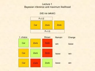
MONTE HALL Should we switch the door or stay?????
A contestant chose door 1 and then the host opened one of the other doors(door 3). Would switching from door 1 to door 2 increase chances of winning the car? http://en.wikipedia.org/wiki/Monty_Hall_problem
={Door i conceals a car} ={Host opens Door j after a contestant choose Door1} (when you stay) (when you switch)