Download
1 / 18
180 likes | 323 Vues
Exploring 3D Power Distribution Network Physics. Xiang Hu 1 , Peng Du 2 , and Chung-Kuan Cheng 2 1 ECE Dept., 2 CSE Dept., University of California, San Diego 10/25/2011. Outline. Introduction 3D power distribution network (PDN) model Circuit model Current model 3D PDN analysis flow

E N D
Exploring 3D Power Distribution Network Physics Xiang Hu1, Peng Du2, and Chung-Kuan Cheng2 1ECE Dept., 2CSE Dept., University of California, San Diego 10/25/2011
Outline • Introduction • 3D power distribution network (PDN) model • Circuit model • Current model • 3D PDN analysis flow • Experimental results • On-chip Current Distribution • Resonance phenomena • Noise reduction techniques • Larger decap around TSVs • Reduce Tier to tier impedance • Conclusions
Introduction • Power delivery issues in 3D ICs • More tiers => More current • Same footprint on package • TSVs and µbumps between tiers • Coarse power grid models • Missed detailed metal layer information • Current source models • Detailed 3D PDN analysis • Frequency domain: resonance behavior • Time domain: worst-case noise
3D PDN Circuit and Current Models • Circuit Model • Lump model: Two-port model for chip between tiers • Fine grid model: all metal layers: m1+ • Current Model • Power law • Phase in f domain
3D PDN Distributed Model[1] • Power grid • Structure: M1, M3, M6, RDL • Each layer extracted in Q3D • T2T: TSV+μbump • Modeled as an RLC element • Package: C4 bump based RLC model [1] X. Hu et al., “Exploring the Rogue Wave Phenomenon in 3D Power Distribution Networks,” IEEE 19th Conf. on Electrical Performance of Electronic Packaging and Systems, Oct. 2010, pp. 57–60.
Frequency-Domain Current Stimulus Model • Noise depends on the current model • Rents rule power law: • P: power consumption • A: area • k: constant number • γ: exponent of the power law • Current configurations • γ =0: single current load • 0< γ <1: taper-shaped current distribution • γ =1: uniform current distribution • In f domain, we can tune the phase
Experiment Base Setup • Two-tier PDN • TSV setup: 3x4 TSVs connected to M1 and AP on both side • 5nF/mm2 decap on T1; 50nF/mm2 decap on T2 • 2x2 C4 on T1 AP • Per bump inductance: 210pH • Per bump resistance: 18.7mΩ
Current Model: Input on T1 • Two-tier PDN + VRM, board, and package • Decap: 5nF/mm2@T1; 50nF/mm2@T2 • Current: T1; distr.(γ=0, 0.5, 1) • Probe • A: T1 TSVs • B: T1 between TSVs • C: T2 • Observation • Smaller γ => larger noise • Resonance at non-TSVs, but not at TSVs T1-T2 brd-pkg VRM-brd
Current Model: Noise Map w/ Input on T1 (@1GHz) γ=1 γ=0.05 T1 γ=0 T2
Current Model: Input on T2 • Two-tier PDN + VRM, board, and package • Decap: 5nF/mm2@T1; 50nF/mm2@T2 • Current: T2; distr.(γ=0, 0.5, 1) • Probe • A: T1 TSV location • B: T1 non-TSV location • C: T2 • Observation • Smaller γ => larger noise
Current Model: Noise Map w/ Input @T2 (1GHz) γ=1 γ=0 γ=0.05 T1 T2
Resonance Phenomena • Decap: 5nF/mm2 @T1; 50nF/mm2 @T2 • Current: T1 or T2, unif. (γ=1) • Observation: resonance vary with decap configurations Probe: T1 Current: T1 Probe: T2 Current: T2 Global mid-freq resonance peak @ non-TSV locations. From lumped model: No mid-freq resonance peak due to “Rm1” No resonance peak @ TSV locations
Decap: Larger Decap Around TSVs • Decap: 50nF/mm2@T1; 5nF/mm2@T2 • Case 1: uniform distribution @T1 • Case 2: half of decap at TSVs @T1 • Observation: Case 2 is better Probe: T1 between TSVs Current: T1 unif. Probe: T2 Current: T2, unif Probe: T2 Current: T1 unif
Tier to Tier Impedance: Number of TSVs TSV Setup
Tier to Tier Impedance: Number of TSVs • TSV(Xpitch,Ypitch) • Case 1: (40, 100) • Case 2: (20, 40) • Case 3: (15, 18) • Current: T1, unif. (γ=1) • Probes • A: T1 TSV • B: T1 between TSVs • C: T2 • Observation • noise drops as #TSV increases • resonance f drops as #TSV increases Resonant f determined by Cd1 As T2T impedance becomes smaller, resonance frequency is determined by both Cd1 and Cd2
Conclusion • On-chip power network model • Current distribution model • Power law current distribution model reflects the current-area relation • Decap: Various on-chip resonances • Techniques of reducing 3D PDN noise • Larger decap around TSV area • Small tier to tier impedance