Download
1 / 20
200 likes | 310 Vues
Exploring the Rogue Wave Phenomenon in 3D Power Distribution Networks. Xiang Hu 1 , Peng Du 2 , Chung-Kuan Cheng 2 1 ECE Dept., 2 CSE Dept. University of California, San Diego 10/25/2010. Agenda. Introduction System-level 3D PDN analysis Chip-level 3D PDN analysis

E N D
Exploring the Rogue Wave Phenomenon in 3D PowerDistribution Networks Xiang Hu1, Peng Du2, Chung-Kuan Cheng2 1ECE Dept., 2CSE Dept. University of California, San Diego 10/25/2010
Agenda • Introduction • System-level 3D PDN analysis • Chip-level 3D PDN analysis • Detailed 3D power grid model • Frequency-domain analysis • Time-domain analysis • Conclusions
Introduction • Power delivery issues in 3D ICs • Total currents flowing through off-chip components increase with the number of stacked tiers • 3D-related components (i.e., TSV, µbump) add more impedance to on-chip power grids • Previous power grid models for on-chip noise analysis are relatively simple • Missed detailed metal layer information • Not suitable for 3D PDN analysis • Detailed 3D PDN analysis has not been done • Frequency domain: resonance behavior • Time domain: worst-case noise
System-Level 3D PDN model • Power delivery system including VRM, board and package • Multiple input current sources Zext
Impedance Profiles in System-Level 3D PDN Model • Common resonant peaks at VRM-board, board-package, and package-T1 interfaces. • No high-frequency peak for Z11. • High-frequency peak for Z22 due to T1-T2 resonance. • Small high-frequency bumps for Z12 and Z21 due to T1-T2 resonance. pkg-T1 T1-T2 VRM-brd brd-pkg
Chip-Level 3D Power Grid Model • Power grid • structure: M1, M3, M7, RDL • Extracted in Q3D • TSV: RLC model • Package: distributed RLC model
Current Source @ T1, Output Voltage @ T1 2D PDN vs. 3D PDN • Measured on-chip impedance on device layer, i.e., M1 • 2D PDN • Large impedance at low frequencies due to high resistive M1 • Only one resonance peak at package-die interface • 3D PDN • Small impedance at low frequencies due to low resistive RDL on T2 • Mid-frequency resonance peak at package-die interface • Large high-frequency resonance peak around T2T location 243.59MHz 241.73MHz Estimated package-die resonant frequency
Current Source @ T1, Output Voltage @ T1 • High-frequency resonance peak • Caused by the inductance of T2T connection and the local decoupling capacitance around it. • Highly-localized: beyond 40um the peak disappears (bypassed by other decaps around the current source) 23.62GHz Single TSV inductance: 34pH Local capacitance on M1: 1.159pF Estimated resonant frequency: 25.4GHz
Current Source @ T1, Output Voltage @ T2 • Small low-frequency impedance • Global mid-frequency resonance peak at package-T1 interface • Global high-frequency resonance peak at T1-T2 interface pkg-T1: 245.5MHz Effective TSV inductance: 2.83pH Total capacitance on T2: 25.96pF Estimated resonant frequency: 18.56GHz T1-T2: 20.26GHz
Current Source @ T2, Output Voltage @ T2 • Large impedance at current source location due to high-resistive M1 • Global mid-frequency resonance peak at package-T1 interface • Caused by the anti-resonance between package inductance and total on-chip capacitance • Global high-frequency resonance peak at T1-T2 interface • Caused by the anti-resonance between T2T inductance and T2 total capacitance
Current Source @ T2, Output Voltage @ T1 • Large impedance at T2T locations • T2 current concentrates on the limited number of T2T locations • Local high-frequency resonance peak at T2T locations • Global mid-frequency resonance peak at package-T1 interface
On-Chip Worst-Case PDN Noise Prediction Algorithm • Motivation • Local current on M1 is tiny consider the distributed current effect • Obtain worst-case noise at multiple on-chip locations • Single-input worst-case PDN noise prediction algorithm [1] • Basic idea: dynamic programming • Multi-input worst-case PDN noise prediction algorithm • Extension of the single-input algorithm • Based on noise superimposition of the linear PDN model [1] P. Du, X. Hu, S. H. Weng, A. Shayan, X. Chen, A. E. Engin, and C.K Cheng. “Worst-Case Noise Prediction With Non-Zero Current Transition Times for Early Power Distribution System Verification,” In IEEE International Symposium on Quality Electronic Design, 2010
On-Chip Worst-Case PDN Noise Flow Current source locations Pick one current source PDN netlist Simulate impulse responses All current sources traversed? Select an output node Current constraints Calculate the worst-case noise More output nodes? Worst-case noise map
Worst-Case Noise Experiment Setting • Two-tier 3D PDN • 9 uniformly distributed current sources on each tier • Same (x,y) current source locations on two tiers • First and last columns of the current sources locate at the same (x,y) coordinates as T2T connections • Current constraints • Maximum amplitude: 0.1mA • Minimum transition time: 10ps
Worst-Case Noise Map on T1 • Currents from T2 cause large noise around T2T interface. • Currents at T2T locations on T1 cause local high-frequency resonance peaks, making the noise worse. peak value
Worst-Case Noise Map on T2 • Uniform worst-case noise peak at nine current source locations • T2T distribution has no impact on the worst-case noise peak distributions on T2 • Worst-case noise on T2 is 20 times of that on T1 peak value
Rogue Waves: Time-Domain Worst-Case Noise Waveforms • Three output locations: • Blue: T2T location on T1 • Red: Away from T2T locations on T1 • Black: T2 • Worst-case noise response: low-frequency oscillations followed by high-frequency oscillations Rogue Wave • Worst-case noise response is dependent on the resonance behaviors of the output nodes and the spatial distribution of current sources • Output nodes on T2 (black): high-frequency oscillation followed by low-frequency oscillation due to global high-frequency resonance • Output nodes on T1 • T2T location (blue): high-frequency oscillation followed by low-frequency oscillation due to local high-frequency resonance • Away from T2T (red): no high-frequency oscillation
Worst-Case Noise Flow Run Time N: number of current sources M: number of output nodes
Conclusions • System-level analysis reveals the global resonance effects for 3D PDNs • Proposed on-chip 3D power grid model with detailed metal layer • Local resonance phenomenon due to T2T connection inductance and local capacitance is discovered with the detailed 3D power grid model • Worst-case noise calculation algorithm is extended to multiple input multiple output system • Worst-case noise map shows the spatial distribution of the worst-case noise in 3D PDNs • The “rogue wave” of worst-case noise response reflects the resonance behaviors at different locations of the 3D PDN