Download
1 / 19
190 likes | 307 Vues
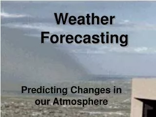
Air Pollution Potential and Fire Weather Forecasting. Anthony R. Lupo Atms Sci 4310 / 7310 Lab 9. Air Pollution Potential Forecasting. Q: Who is interested in this? Why should I be?

E N D
Air Pollution Potential and Fire Weather Forecasting Anthony R. Lupo Atms Sci 4310 / 7310 Lab 9
Air Pollution Potential Forecasting • Q: Who is interested in this? Why should I be? • A: The general public! Thus, entities like The Weather Channel, Air Quality Monitors (Health, Regulators), Forest Managers, and Government / Private Sector forecasters.
Air Pollution Potential Forecasting • Forecast Philosophy: today, numerical models can provide more detailed analysis of where and when these type of conditions will exist. • Then, forecasts represent conditions for pollution (build-up) potential (air stagnation) not for specific pollutants and/or their concentrations, whether these are manmade or natural pollutants.
Air Pollution Potential Forecasting • Climatology • Eastern US: (east of the Rockies) • Summer (all) and fall (primarily south) are most favorable times for air stagnation. • The fall conditions may represent “Indian Summer”.
Air Pollution Potential Forecasting • Western US (west of Rockies and Rockies): • Can be quite common in the spring (Mar - May).
Air Pollution Potential Forecasting • Favorable meteorological conditions • 1) slow moving surface high pressure, and or ridge aloft, with weak horizontal pressure gradients (height gradients) • 2) light winds in the mixed layer (PBL - planetary boundary layer what’s this?) • 3) stable air the boundary layer (Ge < Gm)
Air Pollution Potential Forecasting • 4) No precipitation! (precipitation will scavenge particulates) • NCEP Air Pollution Stagnation Areas • an area for which ALL the following conditions are met are said to possess a high potential for air stagnation.
Air Pollution Potential Forecasting • A) 850 hPa (5000 ft) windspeeds of less than 10 m/s or 20 kts (Red Flag for fire weather is > 25 kts at the surface) • this suggests a small “ventillation” rate and minimal mechanical mixing. • B) 850 hPa (5000 ft) Temperature change in the past 12 h is less than –5C, or weak advections. • this eliminates the possiblity of strong CAA and a change of airmass to cold/cool and clear.
Air Pollution Potential Forecasting • C) 500 hPa absolute vorticity less than 10 x 10-5 s-1, (recall f = 10 x 10-5 at ~43o N), • this suggests that the relative Vorticity is less than 0, which is indicative of a ridge aloft, preferrably a quasi-stationary long wave ridge. • D) 500 hPa 12 –hr vorticity change of less than 3 x 10⁻⁵ s-2 • this identifies ridges than are not moving very much.
Air Pollution Potential Forecasting • E) Probability of precipitation is less than 45% • F) Red Flag is prolonged periods with less than 15% RH. • this means no surface fronts or particulate scavenging! • If we meet all these criterion, then we issue air stagnation advisories.
Air Pollution Potential Forecasting • Another technique often used is the “mixing height” (Miller – Holzworth) technique: • Higher mixing height would indicate more mixing, and less change of air stagnation (trapping of particles). • We will “calculate” (using empirical methods) a morning and afternoon mixing height and compare this to an empirically derived standard.
Air Pollution Potential Forecasting • Morning mixing height http://www.wrh.noaa.gov/sew/fire/olm/mxhgts.htm: • 1) The height above the ground where the surface temperature + “heat island correction”, following the dry adiabat intersects sounding. • 2) Correction: +3C if the Obs. Site is considered “urban”, (STL), and +5C “rural” (MCI) • 3) Calculate transport wind (tw): (tw) is mean wind speed in the mixing layer.
Air Pollution Potential Forecasting • The criterion: • If the morning mixing height is less than 500 m (1640 ft) and a mean wind of less than 4 m/s (8kts), this is significant. • This indicates poor mixing and dispersion of pollution. • You can convert pressure to height using the hypsometric equation on thermodynamic diagram.
Air Pollution Potential Forecasting • Afternoon mixing height (http://www.wrh.noaa.gov/sew/fire/olm/mxhgts.htm): • 1) height above the ground at which the dry adiabat following from the maximum temperature (forecast or observed), intersects the sounding. • 2) Transport wind speed is the average wind speed through the afternoon mixing layer
Air Pollution Potential Forecasting • The criterion: • afternoon mixing height of less than 4920 ft and a transport wind speed of less than 4 m/s (8kts) are considered significant. Calculate height via hypsometric equation.
Air Pollution Potential Forecasting • Ventillation • Ventillation is mixing height x wind speed (in metres) (m2/s) is answer. It is a measure of how fast particles dispersed or removed. • This quantity is often used by fire weather forecasters. • Values of less than 6000 m2/s for 1 to 3 days or 8000 m2/s for more than 2 days are considered significant.
Air Pollution Potential Forecasting • The End!
Air Pollution Potential Forecasting • Questions? • Comments? • Criticisms? • LupoA@missouri.edu