Download
1 / 18
180 likes | 284 Vues
Operational Scheme and Schedule: Basics. Basic scheme (analysis + forecast) Global-Modell (GME, global and synoptic-scale) Lokal Modell (LM, highly resolved mesoscale model) 3 runs per day 00, 12, 18 UTC 03, 06, 09, 15, 21 UTC only analysis Schedule determined by data cut-off

E N D
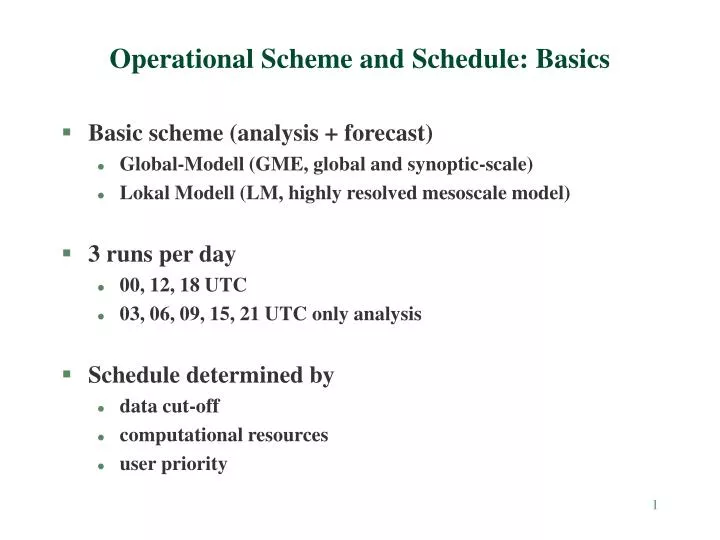
Operational Scheme and Schedule: Basics • Basic scheme (analysis + forecast) • Global-Modell (GME, global and synoptic-scale) • Lokal Modell (LM, highly resolved mesoscale model) • 3 runs per day • 00, 12, 18 UTC • 03, 06, 09, 15, 21 UTC only analysis • Schedule determined by • data cut-off • computational resources • user priority
Boundary values and forecast range • forecast range of LM: 48h • every hour LM gets new boundary data from GME • smooth transition within 8 grid points • continous data assimilation • forecast range of GME • 00, 12 UTC: 174h • 18 UTC: 48h
Schedule of GME/LM-runs (relative to starting time) • +2h 06min start of GME-analysis • +2h 23 min start of LM-analysis • +2h 30 min start of GME-forecast • +2h 34 min start of LM-forecast • +3h 45 min 48h-LM-forecast available • +4h 30 min 174h-GME-forecast available • Postprocessing- • Graphic-files: 5 min • local forecast parameters: 15 min • Availability of final products about 5 hours after starting time
Basic postprocessing • Interpolation between model levels and pressure levels • model level (34m): Typical vertical profiles (depending on stability, e.g) • T 2m • wind 10m • LM-model-levels 26 and 27 for 850-hPa-level, e.g • Reduction of model surface pressure to mean sea level • base: adiabatic gradient • in the case of mountainous areas (e.g. Greenland) • reduced amount of vertical temperature gradient • however, often too high surface pressure values
Postprocessing (further steps) • Automatic weather interpretation • for all fields and local products: describing model weather output of GME and LM • Generation of graphical and alphanumerical products • general analysis and forecast fields • MPEG-files (TriVis) with animations of • cloud development • precipication • wind • temperature • local model output as meteograms and local soundings • local direct model output as alphanumerical information • local output through Kalman, Model Output Statistics and Perfect Prog
Postprocessing (Cross Sections) • Time series of preselected cross-sections of relevant parameters • cloudiness • wind • temperature
Postprocessing (followed-up-models) • Followed-up models (based upon GME-/LM-output) • sea state models • water level (e.g. tides) • waves • trajectory model • pollution (e.g.) • winter road maintenance • SWIS (1-D-model for road surface temperature and road condition) • agro- and biometeorological models • fungus disease • ultraviolett irradiation • test: 1-D-model for fog and low clouds
Computer-system: NWP-runs, IBM • distributed memory massively parrallel processors • application units: 1920 • different model areas are related to different processors • communication between these areas is performed • COS4: 448, COS5: 1472 processor units • memory: 1240 GByte • disk capacity: 7562 GByte • peak performance of each processor unit: 2.4 GFlop/s • „beat frequency“: 375 MHz • each „beat“ : e.g. 8 floating point operations (by considering more bits)!
Computer-system: data storage, communication (I) • 2 IBM p690, each • 32 processors • 128 GB memory • 864 GB disk capacity • tasks (e.g.) • developments, tests • routine jobs (decoding of observations, production of graphics, etc) • data handling • Storage server (e.g., test results) • 3 x 13.5 TByte
Computer-system: data storage, communication (II) • data amount • 174h-GME-run: 40 GByte • 48h-LM-run: 5 GByte • totaly NWP-production > 120 Gbyte per day (follow-up models inclusive ) • Archive (SGI O200) • 24 processors • 24 GB memory • 853 GB disc capacity • archiving of data on cassettes (600 TByte)