Download
1 / 59
610 likes | 1.01k Vues
Lecture III: Collective Behavior of Multi -Agent Systems: Analysis. Zhixin Liu Complex Systems Research Center, Academy of Mathematics and Systems Sciences, CAS. In the last lecture, we talked about. Complex Networks Introduction Network topology Average path length

E N D
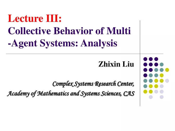
Lecture III:Collective Behavior of Multi -Agent Systems: Analysis Zhixin Liu Complex Systems Research Center, Academy of Mathematics and Systems Sciences, CAS
In the last lecture, we talked about Complex Networks • Introduction • Network topology Average path length Clustering coefficient Degree distribution • Some basic models • Regular graphs: complete graph, ring graph • Random graphs: ER model • Small-world networks: WS model, NW model • Scale free networks: BA model • Concluding remarks
Lecture III:Collective Behavior of Multi -Agent Systems: Analysis Zhixin Liu Complex Systems Research Center, Academy of Mathematics and Systems Sciences, CAS
Outline • Introduction • Model • Theoretical analysis • Concluding remarks
What Is The Agent? From Jing Han’s PPT
What Is The Agent? • Agent:system with two important capabilities: • Autonomy: capable ofautonomous action– of deciding for themselves what they need to do in order to satisfy their objectives; • Interactions: capable of interacting with other agents - the kind of social activity that we all engage in every day of our lives: cooperation, competition, negotiation, and the like. • Examples: Individual, insect, bird, fish, people, robot, … From Jing Han’s PPT
Multi-Agent System (MAS) • MAS • Many agents • Local interactions between agents • Collective behavior in the population level • More is different.---Philp Anderson, 1972 • e.g., Phase transition, coordination, synchronization, consensus, clustering, aggregation, …… • Examples: • Physical systems • Biological systems • Social and economic systems • Engineering systems • … …
Bacteria Colony Flocking of Birds Biological Systems Ant Colony Bee Colony
From Local Rules to Collective Behavior Phase transition, coordination, synchronization, consensus, clustering, aggregation, …… scale-free, small-world pattern A basic problem: How locally interacting agents lead to the collective behavior of the overall systems? swarm intelligence Crowd Panic
Outline • Introduction • Model • Theoretical analysis • Concluding remarks
Modeling of MAS • Distributed/Autonomous • Local interactions/rules • Neighbors may be dynamic • May have no physical connections
A Basic Model This lecture will mainly discuss
Assumption Each agent • makes decision according to local information ; • has the tendency to behave as other agents do in its neighborhood.
r Alignment:steer towards the average heading of neighbors A bird’s Neighborhood Vicsek Model(T. Vicsek et al. , PRL, 1995) http://angel.elte.hu/~vicsek/ Motivation: to investigate properties in nonequilibrium systems A simplified Boid model for flocking behavior.
r Notations xi(t) : position of agent i in the plane at time t : heading of agent i, i= 1,…,n. t=1,2, …… v: moving speed of each agent r: neighborhood radius of each agent Neighbors:
Heading: Position: Vicsek Model Neighbors:
Position: Vicsek Model Neighbors: Heading:
Position: Vicsek Model Neighbors: Heading: is the weighted average matrix.
Vicsek Model http://angel.elte.hu/~vicsek/
Some Phenomena Observed(Vicsek, et al. Physical Review Letters, 1995) a)ρ= 6, ε= 1 high density, large noisec ) b)ρ= 0.48, ε= 0.05 small density, small noise d)ρ= 12, ε= 0.05 higher density, small noise n = 300 v = 0.03 r = 1 Random initial conditions
Synchronization • Def. 1: We say that a MAS reach synchronization if there exists θ, such that the following equations hold for all i, • Question: Under what conditions, the whole system can reach synchronization?
Outline • Introduction • Model • Theoretical analysis • Concluding remarks
(0) (1) (2) (t-1) (t) G(0) G(1) G(2) G(t-1) …… …… x(0) x(1) x (2) x (t-1) x (t) Interaction and Evolution …… …… • Positions and headings are strongly coupled • Neighbor graphs may change with time
Some Basic Concepts If i ~ j Adjacencymatrix: Otherwise Degree: Volume: Degree matrix: Average matrix: Laplacian:
Connectivity of The Graph Connectivity: There is a path between any two vertices of the graph.
G1 G2 G1∪G2 JointConnectivity of Graphs Joint Connectivity: The union of {G1,G2,……,Gm} is a connected graph.
Product of Stochastic Matrices Stochasticmatrix A=[aij]: If ∑jaij=1; and aij≥0 SIA (Stochastic, Indecomposable, Aperiodic) matrix A If where Theorem 1:(J. Wolfowitz, 1963) Let A={A1,A2,…,Am}, if for each sequence Ai1, Ai2, …Aik of positive length, the matrix product AikAi(k-1)…Ai1 is SIA. Then there exists a vector c, such that
The Linearized Vicsek Model A. Jadbabaie , J. Lin, and S. Morse, IEEE Trans. Auto. Control, 2003.
Theorem 2(Jadbabaie et al. , 2003) Joint connectivity of the neighbor graphs on each time interval [th, (t+1)h] with h >0 Synchronization of the linearized Vicsek model Related result: J.N.Tsitsiklis, et al., IEEE TAC, 1984
The Vicsek Model Theorem 3: If the initial headings belong to(-/2, /2), and the neighbor graphs are connected, then the system will synchronize. • Liu and Guo (2006CCC), Hendrickx and Blondel (2006). • The constraint on the initial heading can not be removed.
Connected all the time, but synchronization does not happen. • Differences between with VM and LVM.
The neighbor graph does not converge May not likely to happen for LVM
How to guarantee connectivity? • What kind of conditions on model parameters are needed ?
Random Framework Random initial states: 1) The initial positions of all agents are uniformly and independently distributed in the unit square; 2) The initial headings of all agents are uniformly and independently distributed in [-+ε, -ε] with ε∈(0, ).
Random Graph G(n,p): all graphs with vertex set V={1,…,n} in which the edges are chosen uniformly and independently with probability p. , then Theorem5Let Corollary: Not applicable to neighbor graph ! P.Erdős,and A. Rényi (1959)
Random geometric graph: If are i.i.d. in unit cube uniformly, then geometric graph is called a random geometric graph Random Geometric Graph Geometric graphG(V,E): *M.Penrose, Random Geometric Graphs, Oxford University Press,2003.
Connectivity of Random Geometric Graph Theorem6 Graph with is connected with probability one as if and only if ( P.Gupta, P.R.Kumar,1998 )
Analysis of Vicsek Model • How to deal with changing neighbor graphs ? • How to estimate the rate of the synchronization? • How to deal with matrices with increasing dimension? • How to deal with the nonlinearity of the model?
Projection onto the subspace spanned by Dealing With Graphs With Changing Neighbors 2) Stability analysis of TV systems (Guo, 1994) 3) Estimation of the number of agents in a ring
Estimating the Rate of Synchronization The rate of synchronization depends on the spectral gap. Normalized Laplacian: Spectrum : Spectral gap: Rayleigh quotient
Example: = + Lemma 2:For large n, we have The Upper Bound of Lemma1:Let edges of all triangles be “extracted” from a complete graph. Then there exists an algorithm such that the number of residual edges at each vertex is no more than three. ( G.G.Tang, L.Guo, JSSC, 2007 )
The Lower Bound of Lemma 3: For an undirected graph G, suppose there exists a path set P joining all pairs of vertexes such that each path in P has a length at most l, and each edge of G is contained in at most m paths in P. Then we have Lemma 4: For random geometric graphs with large n , ( G.G.Tang, L.Guo, 2007 )
The Lower Bound of ( G.G.Tang, L.Guo, 2007 )
Estimating The Spectral Gap of G(0) Proposition 1:For G(n,r(n)) with large n ( G.G.Tang, L.Guo, 2007 )
Moreover, if then we have Analysis of Matrices with Increasing Dimension Estimation of multi-array martingales where
Analysis of Matrices with Increasing Dimension Using the above corollary, we have for large n
Dealing With Inherent Nonlinearity A key Lemma:There exists a positive constantη, such that for large n, we have : with