Download

1 / 26
270 likes | 480 Vues
Nearest Neighbour Condensing and Editing. David Claus February 27, 2004 Computer Vision Reading Group Oxford. Nearest Neighbour Rule. Non-parametric pattern classification. Consider a two class problem where each sample consists of two measurements ( x,y ).

E N D
Nearest NeighbourCondensing and Editing David Claus February 27, 2004 Computer Vision Reading Group Oxford
Nearest Neighbour Rule Non-parametric pattern classification. Consider a two class problem where each sample consists of two measurements (x,y). For a given query point q, assign the class of the nearest neighbour. k = 1 Compute the k nearest neighbours and assign the class by majority vote. k = 3
Example: Digit Recognition • Yann LeCunn – MNIST Digit Recognition • Handwritten digits • 28x28 pixel images: d = 784 • 60,000 training samples • 10,000 test samples • Nearest neighbour is competitive
Nearest Neighbour Issues • Expensive • To determine the nearest neighbour of a query point q, must compute the distance to all N training examples • Pre-sort training examples into fast data structures (kd-trees) • Compute only an approximate distance (LSH) • Remove redundant data (condensing) • Storage Requirements • Must store all training data P • Remove redundant data (condensing) • Pre-sorting often increases the storage requirements • High Dimensional Data • “Curse of Dimensionality” • Required amount of training data increases exponentially with dimension • Computational cost also increases dramatically • Partitioning techniques degrade to linear search in high dimension
Questions • What distance measure to use? • Often Euclidean distance is used • Locally adaptive metrics • More complicated with non-numeric data, or when different dimensions have different scales • Choice of k? • Cross-validation • 1-NN often performs well in practice • k-NN needed for overlapping classes • Re-label all data according to k-NN, then classify with 1-NN • Reduce k-NN problem to 1-NN through dataset editing
Exact Nearest Neighbour • Asymptotic error (infinite sample size) is less than twice the Bayes classification error • Requires a lot of training data • Expensive for high dimensional data (d>20?) • O(Nd) complexity for both storage and query time • N is the number of training examples, d is the dimension of each sample • This can be reduced through dataset editing/condensing
Decision Regions Each cell contains one sample, and every location within the cell is closer to that sample than to any other sample. A Voronoi diagram divides the space into such cells. Every query point will be assigned the classification of the sample within that cell. The decision boundary separates the class regions based on the 1-NN decision rule. Knowledge of this boundary is sufficient to classify new points. The boundary itself is rarely computed; many algorithms seek to retain only those points necessary to generate an identical boundary.
Condensing • Aim is to reduce the number of training samples • Retain only the samples that are needed to define the decision boundary • This is reminiscent of a Support Vector Machine • Decision Boundary Consistent – a subset whose nearest neighbour decision boundary is identical to the boundary of the entire training set • Minimum Consistent Set – the smallest subset of the training data that correctly classifies all of the original training data Original data Condensed data Minimum Consistent Set
Condensing • Condensed Nearest Neighbour (CNN) Hart 1968 • Incremental • Order dependent • Neither minimal nor decision boundary consistent • O(n3) for brute-force method • Can follow up with reduced NN [Gates72] • Remove a sample if doing so does not cause any incorrect classifications • Initialize subset with a single training example • Classify all remaining samples using the subset, and transfer any incorrectly classified samples to the subset • Return to 2 until no transfers occurred or the subset is full
Condensing • Condensed Nearest Neighbour (CNN) Hart 1968 • Incremental • Order dependent • Neither minimal nor decision boundary consistent • O(n3) for brute-force method • Can follow up with reduced NN [Gates72] • Remove a sample if doing so does not cause any incorrect classifications • Initialize subset with a single training example • Classify all remaining samples using the subset, and transfer any incorrectly classified samples to the subset • Return to 2 until no transfers occurred or the subset is full
Condensing • Condensed Nearest Neighbour (CNN) Hart 1968 • Incremental • Order dependent • Neither minimal nor decision boundary consistent • O(n3) for brute-force method • Can follow up with reduced NN [Gates72] • Remove a sample if doing so does not cause any incorrect classifications • Initialize subset with a single training example • Classify all remaining samples using the subset, and transfer any incorrectly classified samples to the subset • Return to 2 until no transfers occurred or the subset is full
Condensing • Condensed Nearest Neighbour (CNN) Hart 1968 • Incremental • Order dependent • Neither minimal nor decision boundary consistent • O(n3) for brute-force method • Can follow up with reduced NN [Gates72] • Remove a sample if doing so does not cause any incorrect classifications • Initialize subset with a single training example • Classify all remaining samples using the subset, and transfer any incorrectly classified samples to the subset • Return to 2 until no transfers occurred or the subset is full
Condensing • Condensed Nearest Neighbour (CNN) Hart 1968 • Incremental • Order dependent • Neither minimal nor decision boundary consistent • O(n3) for brute-force method • Can follow up with reduced NN [Gates72] • Remove a sample if doing so does not cause any incorrect classifications • Initialize subset with a single training example • Classify all remaining samples using the subset, and transfer any incorrectly classified samples to the subset • Return to 2 until no transfers occurred or the subset is full
Condensing • Condensed Nearest Neighbour (CNN) Hart 1968 • Incremental • Order dependent • Neither minimal nor decision boundary consistent • O(n3) for brute-force method • Can follow up with reduced NN [Gates72] • Remove a sample if doing so does not cause any incorrect classifications • Initialize subset with a single training example • Classify all remaining samples using the subset, and transfer any incorrectly classified samples to the subset • Return to 2 until no transfers occurred or the subset is full
Condensing • Condensed Nearest Neighbour (CNN) Hart 1968 • Incremental • Order dependent • Neither minimal nor decision boundary consistent • O(n3) for brute-force method • Can follow up with reduced NN [Gates72] • Remove a sample if doing so does not cause any incorrect classifications • Initialize subset with a single training example • Classify all remaining samples using the subset, and transfer any incorrectly classified samples to the subset • Return to 2 until no transfers occurred or the subset is full
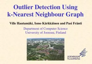
Proximity Graphs • Condensing aims to retain points along the decision boundary • How to identify such points? • Neighbouring points of different classes • Proximity graphs provide various definitions of “neighbour” NNG = Nearest Neighbour Graph MST = Minimum Spanning Tree RNG = Relative Neighbourhood Graph GG = Gabriel Graph DT = Delaunay Triangulation
Proximity Graphs: Delaunay • The Delaunay Triangulation is the dual of the Voronoi diagram • Three points are each others neighbours if their tangent sphere contains no other points • Voronoi editing: retain those points whose neighbours (as defined by the Delaunay Triangulation) are of the opposite class • The decision boundary is identical • Conservative subset • Retains extra points • Expensive to compute in high dimensions
Proximity Graphs: Gabriel • The Gabriel graph is a subset of the Delaunay Triangulation • Points are neighbours only if their (diametral) sphere of influence is empty • Does not preserve the identical decision boundary, but most changes occur outside the convex hull of the data points • Can be computed more efficiently Green lines denote “Tomek links”
Proximity Graphs: RNG • The Relative Neighbourhood Graph (RNG) is a subset of the Gabriel graph • Two points are neighbours if the “lune” defined by the intersection of their radial spheres is empty • Further reduces the number of neighbours • Decision boundary changes are often drastic, and not guaranteed to be training set consistent Gabriel edited RNG edited – not consistent
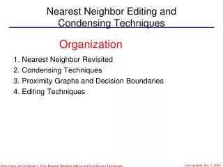
Dataset Reduction: Editing • Training data may contain noise, overlapping classes • starting to make assumptions about the underlying distributions • Editing seeks to remove noisy points and produce smooth decision boundaries – often by retaining points far from the decision boundaries • Results in homogenous clusters of points
Wilson Editing • Wilson 1972 • Remove points that do not agree with the majority of their k nearest neighbours Earlier example Overlapping classes Original data Original data Wilson editing with k=7 Wilson editing with k=7
Multi-edit • Diffusion: divide data into N ≥ 3 random subsets • Classification: Classify Si using 1-NN with S(i+1)Mod N as the training set (i = 1..N) • Editing: Discard all samples incorrectly classified in (2) • Confusion: Pool all remaining samples into a new set • Termination: If the last I iterations produced no editing then end; otherwise go to (1) • Multi-edit [Devijer & Kittler ’79] • Repeatedly apply Wilson editing to random partitions • Classify with the 1-NN rule • Approximates the error rate of the Bayes decision rule Multi-edit, 8 iterations – last 3 same Voronoi editing
Combined Editing/Condensing • First edit the data to remove noise and smooth the boundary • Then condense to obtain a smaller subset
Where are we? • Simple method, pretty powerful rule • Can be made to run fast • Requires a lot of training data • Edit to reduce noise, class overlap • Condense to remove redundant data
Questions • What distance measure to use? • Often Euclidean distance is used • Locally adaptive metrics • More complicated with non-numeric data, or when different dimensions have different scales • Choice of k? • Cross-validation • 1-NN often performs well in practice • k-NN needed for overlapping classes • Re-label all data according to k-NN, then classify with 1-NN • Reduce k-NN problem to 1-NN through dataset editing