Download
1 / 35
350 likes | 502 Vues
No Distributional Assumption Training Distribution is the same as the Test Distribution Generalization bounds depend on this view and affects model selection . Err D (h) < Err TR (h) + P(VC(H), log(1/ ± ),1/m) This is also called the

E N D
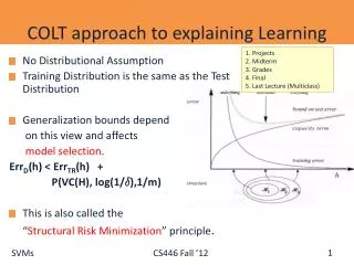
No Distributional Assumption Training Distribution is the same as the Test Distribution Generalization bounds depend on this view and affects model selection. ErrD(h) < ErrTR(h) + P(VC(H), log(1/±),1/m) This is also called the “Structural Risk Minimization” principle. COLT approach to explaining Learning 1. Projects 2. Midterm 3. Grades 4. Final 5. Last Lecture (Multiclass)
No Distributional Assumption Training Distribution is the same as the Test Distribution Generalization bounds depend on this view and affect model selection. ErrD(h) < ErrTR(h) + P(VC(H), log(1/±),1/m) As presented, the VC dimension is a combinatorial parameter that is associated with a class of functions. We know that the class of linear functions has a lower VC dimension than the class of quadratic functions. But, this notion can be refined to depend on a given data set, and this way directly affect the hypothesis chosen for a given data set. COLT approach to explaining Learning
Consider the class of linear functions that separate the data S with margin °. Note that although both classifiers (w’s) separate the data, they do it with a different margin. Intuitively, we can agree that: Large Margin Small VC dimension Data Dependent VC dimension
Theorem (Vapnik): If H°is the space of all linear classifiers in <n that separate the training data with margin at least °, then VC(H°) · R2/°2 where R is the radius of the smallest sphere (in <n) that contains the data. This is the first observation that will lead to an algorithmic approach. Margin and VC dimension
This discussion motivates the notion of a maximal margin. The maximal margin of a data set S is define as: °(S) = max||w||=1 min(x,y) 2 S y wT x Maximal Margin 1. For a given w: Find the closest point. 2. Then, find the one the gives the maximal margin value across all w’s (of size 1). Note: the selection of the point in the min and therefore the max does not change if we scale w, so it’s okay to only deal with normalized w’s.
Theorem (Vapnik): If H°is the space of all linear classifiers in <n that separate the training data with margin at least °, then VC(H°) · R2/°2 where R is the radius of the smallest sphere (in <n) that contains the data. This is the first observation that will lead to an algorithmic approach. The second observationis that: Small ||w|| Large Margin Consequently: the algorithm will be: from among all those w’s that agree with the data, find the one with the minimal size ||w|| Margin and VC dimension
Hard SVM • We want to choose the hyperplane that achieves the largest margin. That is, given a data set S, find: • w* = argmax||w||=1min(x,y) 2 S y wT x • How to find this w*? • Claim: Define w0to be the solution of the optimization problem: w0 = argmin {||w||2 : 8 (x,y) 2 S, y wTx ¸ 1 }. Then: w 0/||w0|| = argmax||w||=1 min(x,y) 2 S y wT x That is, the normalization of w0corresponds to the largest margin separating hyperplane. 1. For a given w: Find the closest point. 2. Among all w’s (of size 1) find the w the maximizes this point’s margin. Note: the selection of the point in the min and therefore w*does not change if we scale w, so it’s okay to only deal with normalized w’s. 1. Consider the set of “good” w’s (those that separate the data). 2. Among those, choose the one with minimal size.
Hard SVM (2) • Claim: Define w0 to be the solution of the optimization problem: w0 = argmin {||w||2 : 8 (x,y) 2 S, y wT x ¸ 1 } (**) Then: w 0/||w0|| = argmax||w||=1 min(x,y) 2 S y wT x That is, the normalization of w0corresponds to the largest margin separating hyperplane. • Proof: Define w’ = w 0/||w0|| and let w*be the largest-margin separating hyperplane. We need to show that w’ = w*. Note first that w*/°(S) satisfies the constraints in (**); therefore: ||w0|| · ||w*/°(S)|| = 1/°(S) . • Consequently: 8 (x,y) 2 S y w’T x = 1/||w0|| y w0Tx ¸1/||w0|| ¸°(S) But since ||w’|| = 1 this implies that w’ corresponds to the largest margin, that is w’= w* Prev. ineq. Def. of w’ Def. of w0
Hard SVM Optimization • We have shown that the sought after weight vector w is the solution of the following optimization problem: SVM Optimization: (***) • Minimize: ½ ||w||2 Subject to:8(x,y) 2S: y wT x ¸ 1 • This is an optimization problem in (n+1) variables, with |S|=m inequality constraints.
Support Vector Machines • The name “Support Vector Machine” stems from the fact that w* is supported by (i.e. is the linear span of) the examples that are exactly at a distance 1/||w*|| from the separating hyperplane. These vectors are therefore called support vectors. • Theorem: Let w* be the minimizer of the SVM optimization problem (***) for S = {(xi, yi)}. Let I= {i: w*Tx = 1}. Then there exists coefficients ®i >0 such that: w* = i2 I®iyixi This representation should ring a bell…
Duality • This, and other properties of Support Vector Machines are shown by moving to the dual problem. • Theorem: Let w* be the minimizer of the SVM optimization problem (***) for S = {(xi, yi)}. Let I= {i: w*Tx = 1}. Then there exists coefficients ®i >0 such that: w* = i2 I®iyixi
Computational Issues Training of an SVM used to be is very time consuming – solving quadratic program. Modern methods are based on Stochastic Gradient Descent Is it really optimal? Is the objective function we are optimizing the “right” one? Key Issues
17,000 dimensional context sensitive spelling Histogram of distance of points from the hyperplane Real Data In practice, even in the separable case, we may not want to depend on the points closest to the hyperplane but rather on the distribution of the distance. If only a few are close, maybe we can dismiss them. This applies both to generalization bounds and to the algorithm.
Soft SVM • Notice that the relaxation of the constraint: yiwitxi¸ 1 • Can be done by introducing a slack variable » (per example) and requiring: yiwitxi¸ 1 - »i; »i¸ 0 • Now, we want to solve: Min ½ ||w||2+ c »isubject to »i¸ 0 • Which can be written as: Min ½ wTw+ c max(0, 1 – yiwitxi). • What is the interpretation of this?
Soft SVM (2) • The hard SVM formulation assumes linearly separable data. • A natural relaxation: maximize the margin while minimizing the # of examples that violate the margin (separability) constraints. • However, this leads to non-convex problem that is hard to solve. • Instead, move to a surrogate loss function that is convex. • SVM relies on the hinge loss function (note that the dual formulation can give some intuition for that too). Minw ½ ||w||2 + c (x,y) 2 S max(0, 1 – y wtx) • where the parameter c controls the tradeoff between large margin (small ||w||) and small hinge-loss.
The problem we solved is: Min ½ ||w||2+ c »i Where »i> 0 is called a slack variable, and is defined by: »i= max(0, 1 – yiwtxi) Equivalently, we can say that: yiwtxi¸ 1 - »; »¸ 0 And this can be written as: Min ½ ||w||2 + c »i General Form of a learning algorithm: Minimize empirical loss, and Regularize (to avoid over fitting) Theoretically motivated improvement over the original algorithm we’ve see at the beginning of the semester. SVM Objective Function Regularization term Empirical loss Can be replaced by other regularization functions Can be replaced by other loss functions
We get an unconstrained problem. We can use the gradient descent algorithm! However, it is quite slow. Many other methods Iterative scaling; non-linear conjugate gradient; quasi-Newton methods; truncated Newton methods; trust-region newton method. All methods are iterative methods, that generate a sequence wkthat converges to the optimal solution of the optimization problem above. Currently: Limited memory BFGS is very popular What Do We Optimize(2)?
1. Earlier methods used Quadratic Programming. Very slow. 2. The soft SVM problem is an unconstrained optimization problems. It is possible to use the gradient descent algorithm! Still, it is quite slow. Many options within this category: Iterative scaling; non-linear conjugate gradient; quasi-Newton methods; truncated Newton methods; trust-region newton method. All methods are iterative methods, that generate a sequence wkthat converges to the optimal solution of the optimization problem above. Currently: Limited memory BFGS is very popular 3. 3rd generation algorithms are based on Stochastic Gradient Decent The runtime does not depend on n=#(examples); advantage when nis very large. Stopping criteria is a problem: method tends to be too aggressive at the beginning and reaches a moderate accuracy quite fast, but it’s convergence becomes slow if we are interested in more accurate solutions. 4. Dual Coordinated Descent (& Stochastic Version) Optimization: How to Solve
Support Vector Machines – Short Summary SVM = Linear Classifier + Regularization + [Kernel Trick]. • Typically we are looking for the best w: wopt = argminw1m L(f(x,w,b),y) Where L is a loss function that penalizes f when it makes a mistake. • Typically, L is the 0-1 loss (hinge-loss): L(y’, y)= ½ |y – sgn y’| (y, y’ 2 {-1,1}) • Just optimizing with respect to the training data may lead to overfitting. We want to achieve good performance on the training while maintaining some notion of “simple” hypothesis. We therefore change our goal to: wopt = argminw1m L(f(x,w,b),y) + R(w) Where L is a loss function, and R is a regularization function, which penalizes w that results in a model that is too complex (high VC dimension). determines the tradeoff between the empirical error and the regularization.
Support Vector Machines – Short Version SVM = Linear Classifier + Regularization + [Kernel Trick]. • This leads to an algorithm: from among all those w’s that agree with the data, find the one with the minimal size ||w|| Minimize ½ ||w||2 Subject to: y(w ¢ x + b) ¸ 1, for all x 2 S • This is an optimization problem that can be solved using techniques from optimization theory. By introducing Lagrange multipliers we can rewrite the dual formulation of this optimization problems as: w = ii yi xi • Where the ’s are such that the following functional is maximized: • L() = -1/2 ij1j xi xj yi yj + ii • The optimum setting of the ’s turns out to be: i yi (w ¢ xi +b -1 ) = 0 8 i
Support Vector Machines – Short Version • Dependence on the dot product leads to the ability to introduce kernels (just like in perceptron) • What if the data is not linearly separable? • What is the difference from regularized perceptron/Winnow? SVM = Linear Classifier + Regularization + [Kernel Trick]. Minimize ½ ||w||2 Subject to: y(w ¢ x + b) ¸ 1, for all x 2 S • The dual formulation of this optimization problems gives: w = iiyi xi • Optimum setting of ’s : iyi (w ¢ xi +b -1 ) = 0 8i • That is, i:=0 only when w ¢ xi +b -1=0 • Those are the points sitting on the margin, call support vectors • We get: f(x,w,b) = w ¢ x +b = iiyi xi¢ x +b • The value of the function depends on the support vectors, and only on their dot product with the point of interest x.
SVM Notes • Chp. 5 of “Support Vector Machine” [Cristianini and Shawe-Taylor] provides an introduction to the theory of Optimization required in order to understand SVMs.
Optimization • We are interested in finding the minimum or a maximum of a function, typically subject to some constraints. • The general problem is: Minimize f(w), w 2 Rn Subject to gi(w) · 0, i=1,…k hi(w) = 0, i=1,…m • An Inequality constraint gi(w) · 0 is called active if the solution w* satisfies gi(w*) = 0 • An inequality constraint can be transformed into an equality constraint by introducing a slack variable: optimization gi(w) · 0 ´ gi(w) + i = 0, ¸ 0 CS446-Spring 10
Optimization Problems • An optimization problem in which the objective function and the constraints are linear is called a linear program. • If the objective function is quadratic and the constraints linear it is called a quadratic program. • If the objective function, the constraints and the domain of the functions are convex, that problem is a convex optimization problem. CS446-Spring 10
f(w) f(u) u w Convexity • A real valued function f(w) is called convex for w 2 Rn if, 8 w,u 2 Rn, and for any a 2 (0,1): f(aw + (1-a)u) · af(w) + (1-a) f(u) • Claim: If a function is convex, any local minimum w* of the unconstrained optimization problem with objective function f is also a global minimum. • Proof: Take any u><w*. By the definition of the local minimum there exists a sufficiently close to 1 that f(w*) · f(aw*+ (1-a)u) · af(w*) + (1-a) f(u) • Where the first inequality is a result of the assumption of local minimum and the second is from the convexity assumption. But that implies (algebra) that f(w*) · f(u) • This is important. It renders optimization problems tractable when the functions involved are convex. CS446-Spring 10
Solving Optimization Problems (1) Theorem 1. A necessary condition for w* to be a minimum of f 2 C, is df(w*)/d(w) =0. This condition, together with convexity, is also a sufficient solution. CS446-Spring 10
Constrained Optimization Problems • Solved by converting constrained problems to unconstrained problems. • When the problems are constrained, there is a need to define the Lagrangian function, which incorporates information about both the objective function and the constraints, and which can be used to detect solutions. • The Lagrangian is defined as the objective function plus a linear combination of the constraints, where the coefficients of the combination are call the Lagrange multipliers. • Given an optimization problem with objective function f(w), and equality constraints hi(w)=0, i=1,…,m, we define the Lagrangian function as: L(w,) = f(w) + i=1mi hi(w) where the coefficients i are called the Lagrange multipliers. CS446-Spring 10
Constrained Optimization Problems (2) • If w* is a local minimum for an optimization problem with only equality constraints, it is possible that df(w*)/d(w) >< 0 (so, w/o constraints it would not be a candidate for extreme point) but that the direction in which we could move to reduce f would violate one or more of the constraints. • In order to respect the equality constraints hi we must move in directions that are perpendicular to dhi(w*)/d(w), that is they do not change the constraints. • Therefore, in order to respect all the constraints we must move perpendicular to the subspace V spanned by: dhi(w*)/dw, (i =1,m) • So, we make the constrained problem be an unconstrained one in which we require that there exists bi such that df(w*)/dw + i=1mi dhi(w*)/dw = 0 CS446-Spring 10
Constrained Optimization Problems (3) Theorem 2 (Lagrange): A necessary condition for w* to be a minimum for an optimization problem with objective f(w) and equality constraints hi (1,…,m) is: df(w*)/dw + i=1mi dhi(w*)/dw = 0 For some values *. These conditions are also sufficient provided that L(w,*) is also a convex function of w. Another way to write it is L(w*,)/dw = L(w*,)/dw =0 The first condition results in a new system of equations. The second, returns the equality constraints. By solving jointly the two systems, one obtains the solution. CS446-Spring 10
Lagrange Theorem: Example • Consider the standard problem of finding the largest volume box with a given surface area. Let the sides of the box be u,v,w. • Optimization problem Minimize: - uvw Subject to: wu+uv+vw=c • The Lagrangian: L = -uvw + (uv+wu+vw-c) • Necessary conditions: • dL/dw= -uv+(u+v); dL/du= -wv+(w+v); dL/dv= -uw+(u+w) • Solving the equations gives v(w-u) = w (u-v) = 0, implying that the only non trivial solution is w=v=u=(c/3)1/2 CS446-Spring 10
Example (Maximum Entropy Distribution) • Suppose we wish to find the discrete probability distribution p= (p1,p2,…pn) with maximal entropy H(p) = -i=1n pi log{pi}. • The optimization problem: minimize -H(p), subject to i=1n pi =1 L(p,) = i=1n pi log{pi} + (i=1n pi -1 ) • Differentiating, we get: log{e pi) + = 0 (i=1,…n) • Which implies that all the pi s are the same p=(1/n…1/n). • It is not hard to show that the function H(p) is convex, so the uniform distribution is the global solution. CS446-Spring 10
General Optimization Problems • We now move to the general case, where the optimization problem contains both equality and inequality constraints. Define the generalize Lagrangian: L(w,, ) = f(w) + i=1ki gi(w) + i=1mi hi(w) Theorem3(Kuhn-Tucker):Given an optimization problem on Rn: Minimize f(w), w 2 Rn Subject to gi(w) · 0, i=1,…k hi(w) = 0, i=1,…m Necessary and sufficient conditions for w* to be an optimum are the existence of *, * such that: dL(w*, *, * )/dw = dL(w*, *, * )/d = 0 And i* gi(w*) = 0 i=1,…,k gi(w*) · 0 i=1,…,k i*¸ 0 i=1,…,k CS446-Spring 10
General Optimization Problems (2) • The last conditions are called KKT: Karush-Kuhn-Tucker conditions. • i* gi(w*) = 0 i=1,…,k gi(w*) · 0 i=1,…,k i*¸ 0 i=1,…,k • It implies that solutions can be in one of two positions with respect to the inequality constraints. • Either the solution is in the interior of the feasible region, so that the constraint is inactive (gi(w*) · 0), or on the boundary defined by that constraints, which is active. In the first case, the i s need to be zero. In the second case, the constraint is active (gi(w*) = 0), and i can be non-zero. This condition will give rise to the notion of support vectors. CS446-Spring 10