Download
1 / 89
1.06k likes | 1.37k Vues
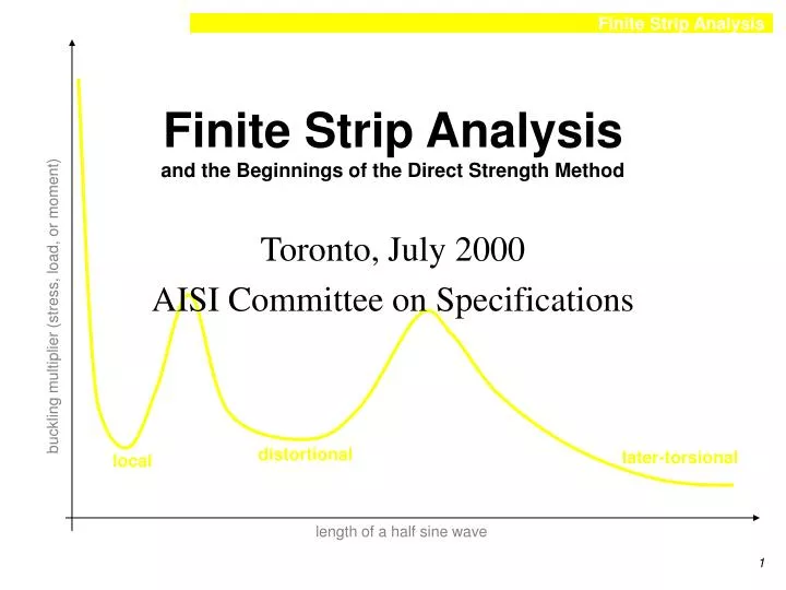
buckling multiplier (stress, load, or moment). distortional. later-torsional. local. length of a half sine wave. Finite Strip Analysis and the Beginnings of the Direct Strength Method. Toronto, July 2000 AISI Committee on Specifications. Overview. Introduction Background

E N D
buckling multiplier (stress, load, or moment) distortional later-torsional local length of a half sine wave Finite Strip Analysisand the Beginnings of the Direct Strength Method Toronto, July 2000 AISI Committee on Specifications
Overview • Introduction • Background • A simple verification problem • Analyze a typical section • Interpreting results (k, fcr, Pcr, Mcr) • Direct Strength Prediction • Improve a typical section • Individual analysis - “do it yourself”
Introduction • Understanding elastic buckling (stress, modes, etc.) is fundamental to understanding the behavior and design of thin-walled structures. • Thorough treatment of plate buckling separates design of cold-formed steel structures from typical structures. • Hand solutions for plate buckling have taken us a great distance but more modern approaches may be utilized now. • Finite strip analysis is one efficient method for calculating elastic buckling behavior.
Introduction • No new theory: Finite strip analysis uses the same “thin plate” theory employed in classical plate buckling solutions (e.g., k = 4) already in current use. • Organized: The nuts and bolts of the analysis is organized in a manner similar to the stiffness method for frames and thus familiar to a growing group of engineers. • Efficient: Single solutions and parameter studies can be performed on PCs • Free: Source code and programs for the finite strip analysis is free
What has to be defined? property give E, G, and v nodes give node number give coordinates indicate if any additional support exist along the longitudinal edge give applied stress on node elements give element number give nodes that form the strip give thickness of the strip lengths give all the lengths that elastic buckling should be examined at
Finite Strip Software • CU-FSM • Matlab based full graphical version • DOS engine only (execufsm.exe) • Helen Chen has written a Windows front end “procefsm.exe” which uses the CU-FSM DOS engine (Thanks Helen!) • Other programs with finite strip capability • THINWALL from University of Sydney • CFS available from Bob Glauz
Overview • Introduction • Background • A simple verification problem • Analyze a typical section • Interpreting results (k, fcr, Pcr, Mcr) • Direct Strength Prediction • Improve a typical section • Individual analysis - “do it yourself”
Theoretical Background • Elastic buckling in matrix form • Initial elastic stiffness [K] • specialized shape functions • Geometric stiffness [Kg] • Forming the solution • Elastic buckling solution
Elastic Buckling (Matrix form) • standard initial elastic stiffness form • consider effect of stress on stiffness • consider linear multiples of constant stress (f1) • eigenvalue problem gives solution
What is [K]? • [K] is the initial elastic stiffness
Shape Functions these shape functions are also known as [N]
Strain-Displacement and [K] Plane stress Kuv comesfrom these strain-displacement relations Bending Kwq comesfrom these strain-displacement relations
What is [Kg]? • [Kg] is the stress dependent geometric stiffness, (compressive stresses erode stiffness) The terms may be derived through • consideration of the total potential energy due to in-plane forces, or • equivalently consider equilibrium in the deformed geometry, (i.e., consider the moments that develop in the deformed geometry due to forces which are in-plane in the undeformed geometry), also • one can consider Kg as a direct manifestation of higher order strain terms.
Developing [Kg] where {d} is the nodal displacementsthe same shape functions as before are used,therefore [G] is determined through partial differentiation of [N].
Forming the Complete Solution • The stiffness matrix for the member is formed by summing the element stiffness matrices (this is done in exactly the same manner as the stiffness solution for frame analysis) • generate stiffness matrices in local coordinates • transform to global coordinates ([k]n=gTk’g) • add contribution of each strip to global stiffness, symbolically:
Eigenvalue Solution • The solution yields • l the multiplier which gives the buckling stress • {d} the buckling mode shapes • The solution is performed for all lengths of interest to develop a complete picture of the elastic buckling behavior
Overview • Introduction • Background • A simple verification problem • Analyze a typical section • Interpreting results (k, fcr, Pcr, Mcr) • Direct Strength Prediction • Improve a typical section • Individual analysis - “do it yourself”
A Simple Verification Problem • Find the elastic buckling stress of a simply supported plate using finite strip analysis. SS SS SS SS width = 6 in. (152 mm) thickness = 0.06 in. (1.52 mm) E = 29500 ksi (203000 MPa) v = 0.3 Hand Solution: = 10.665 ksi
Finite Strip Analysis Notes(analysis of SS plate) • double click procefsm.exe • enter elastic properties into the box • enter the node number, x coordinate, z coordinate, and applied stress • 1,0.0,0.0,1.0 which means node 1 at 0,0 with a stress of 1.0 • 2,6.0,0.0,1.0 which means node 2 at 6,0 with a stress of 1.0 • enter the element number, starting node number, ending node number, number of strips between the nodes (at least 2 typically 4 or more) and the thickness • 1,1,2,2,0.06 which means element 1 goes from node 1 to 2, put 2 strips in there and t=0.06 • select plot cross-section to see the plate • enter a member length (say 6) and number of different half wavelengths (say 10) • do File - Save As - plate.inp • now select view/revise raw data file
Finite Strip Analysis Notes(analysis of SS plate) continued • View/Revise Raw Data File shows the actual text file that is used by the finite strip analysis program. All detailed modifications must be made here before completing the analysis. The format of the file is summarized as: • The x, y, z, q degrees of freedom are shown in the stripto the right. • Supported degrees of freedom are supported along theentire length (edge) of the strip. The ends of the stripare simply supported (due to the selected shapefunctions). Set a DOF variable to 0 to support that DOF along the edge
Finite Strip Analysis Notes(analysis of SS plate) continued • First modify degrees of freedom so the plate is simply supported along the long edges (the loaded edges are always simply supported). Put a pin along the left edge and a roller along the right edge. • 1 0 0 1 1 1 1 1.0 becomes 1 0 0 0 0 1 1 1.0 • 2 3 0 1 1 1 1 1.0 stays the same • 3 6 0 1 1 1 1 1.0 becomes 1 6 0 1 0 1 1 1.0 • Now delete the last line and replace it with the specific lengths that you want to use, say for instance “3 4 5 6 7 8” • Now change the #lengths listed in the thrid column of the first line of the file to match the selected number, in this example we have 6 different lengths • Now select Save for Finite Strip Analysis and save under the name plate.txt • Select Analysis - Open • Then type ‘plate.txt’ for the input file and ‘plate.out’ for the output file • Select Output - then plate.out - and open • Select Plot curve and plot mode, the result of this example is 10.69 ksi (vs. 10.665 ksi hand solution - repeat using 4 strips - then result is 10.666 ksi)
Overview • Introduction • Background • A simple verification problem • Analyze a typical section • Interpreting results (k, fcr, Pcr, Mcr) • Direct Strength Prediction • Improve a typical section • Individual analysis - “do it yourself”
Analyze a typical section • Pure bending of a C • Quickie hand analysis • Finite strip analysis using procefsm.exe • Discussion • Pure compression of a C • Quickie hand analysis • Finite strip analysis • Discussion • Comparisons and Further Discussion
2.44 0.84 8.44 0.059 Strong Axis Bending of a C • Approximate the buckling stress for pure bending. comp. lip comp. flange web
2.44 0.84 8.44 0.059 Strong Axis Bending of a C • Approximate the buckling stress for pure bending. lip flange web * this k value would be fine-tuned by AISI B4.2
Finite Strip Analysis Steps (strong axis bending of a C) • Double click on procefsm.exe • Select File - Open - C.inp • Plot Cross Section • View/Revise Raw Data File • Go to bottom of text file and change lengths to “1 2 3 4 5 6 7 8 9 10 20 30 40 50 60 70 80 90 100” • Go to top of file (1st line 3rd entry) change the number of lengths from 20 to 19 • Save for finite strip analysis as C.txt • Select Analysis - Open - execufsm • Enter in DOS window ‘C.txt’ return then ‘C.out’ • Select output - ‘C.out’ - open • Check 2D, Check undef, push plot mode button • Push plot curve, set half wave-length to 5 rehit plot mode, set to 30 and plot • local buckling at 40ksi (~5 in. 1/2wvlngth), dist buckling at 52ksi (~30 in. 1/2wvlngth)
local buckling distortional local half-wavelength buckling multiplier
Discussion • Finite strip analysis identifies three distinct modes: local, distortional, lateral-torsional • The lowest multiplier for “each mode” is of interest. The mode will “repeat itself” at this half-wavelength in longer members • Higher multipliers of the same mode are not of interest. • The meaning of the“half-wavelength” can bereadily understood fromthe 3D plot. For example:
Discussion • How do I tell different modes? • wavelength: local buckling should occur at wavelengths near or below the width of the elements, longer wavelengths indicate a different mode of behavior • mode shape: in local buckling, nodes at fold lines should rotate only, if they are translating then the local mode is breaking down • What if more minimums occur? • as you add stiffeners and other details more minima may occur, every fold line in the plate adds the possibility of new modes. Definitions of local and distortional buckling are not as well defined in these situations. Use wavelength of the mode to help you decide.
2.44 0.84 8.44 0.059 Compression of a C • Approximate the buckling stress for pure compression. lip flange web * this k value would be fine-tuned by AISI B4.2
Finite Strip Analysis Steps (compression of a C) • Double click on procefsm.exe • Select File - Open - C.inp • Change all applied stress to compression +1.0 • Plot Cross Section • View/Revise Raw Data File • Go to bottom of text file and change lengths to “1 2 3 4 5 6 7 8 9 10 20 30 40 50” • Go to top of file (1st line 3rd entry) change the number of lengths from 20 to 14 • Save for finite strip analysis as C.txt • Select Analysis - Open - execufsm • Enter in DOS window ‘C.txt’ return then ‘C.out’ • Select output - ‘C.out’ - open • Check 2D, Check undef, push plot mode button • Push plot curve, set half wave-length to 6 and rehit plot mode • local buckling at 7.5ksi (pure compression)
Finite Strip AnalysisCompression of a C • fcr local = 7.5 ksi • fcr distortional ~ 20 ksi (this value may be fine tuned by selecting more lengths and re-analyzing) • fcr overall at 80 in. = 29 ksi
Comparision of Elastic Results • Hand Analysis • compression lip=56.6 flange=62.4 web=5.2 ksi • bending lip=56.6 flange=62.4 web=31.3 ksi • Finite strip analysis • compression local=7.5 distortional~20ksi • bending local=40 distortional=52 ksi
Hand Analysis Compression Lip = 56.6 ksi Flange = 62.4 Web = 5.2 Bending Lip = 56.6 Flange = 62.4 Web = 31.3 Finite strip analysis Compression Local = 7.5 ksi Distortional ~ 20 Bending Local = 40 Distortional = 52 Comparision of Results for Buckling Stress of a C
Overview • Introduction • Background • A simple verification problem • Analyze a typical section • Interpreting results (k, fcr, Pcr, Mcr) • Direct Strength Prediction • Improve a typical section • Individual analysis - “do it yourself”
Converting the results • If f1 is the applied stress in the finite strip analysis and l the multiplier that results from the elastic buckling thenfcr = lf1 is known. How do we get k? Pcr? Mcr? • k is found viawhere:b = element width of interest (flange, web, lip etc.) • Pcr = Agfcr • Mcr = Sgfcr(as long as f1 is the extreme fiber stress of interest)
Converting the results - Example • For the C in pure compression what does the finite strip analysis yield for the local buckling k of the web? • For the flange? • Solutions are different when you recognize the interaction!
Converting the results - Example • For the C in compression what is the elastic critical local buckling load? distortional buckling load? overall? • From CU-FSM or hand calculation get the section properties • (Pcr)local = Agfcr = 0.885in2*7.5ksi = 6.6 kips • (Pcr)distortional = Agfcr = 0.885in2*20 ksi = 17.7 kips • (Pcr)overall at 80 in. = Agfcr = 0.885in2*29 ksi = 25.7 kips
Converting the results - Example • For the C in bending what is the elastic critical local buckling moment? distortional buckling moment? • From CU-FSM or hand calculation get the section properties • (Mcr)local = Sgfcr = 2.256in3*40 ksi = 90 in-kips • (Mcr)distortional = Sgfcr = 2.256in3*52 ksi = 117 in-kips
How can I use this information? • Known • local buckling load (Pcr)local from finite strip analysis • distortional buckling load (Pcr)distortional from finite strip analysis • overall or Euler buckling load (Pcr)Euler may be flexural, torsional, or flexural-torsional in the special case of Kx=Ky=Kt then we may use finite strip analysis results, in other cases hand calculations for overall buckling of a column are used • yield load (Py) from hand calculation • Unknown • design capacity Pn • Methodology: Direct Strength Prediction
Overview • Introduction • Background • A simple verification problem • Analyze a typical section • Interpreting results (k, fcr, Pcr, Mcr) • Direct Strength Prediction • Improve a typical section • Individual analysis - “do it yourself”
Direct Strength Prediction • The idea behind Direct Strength prediction is that with (Pcr)local, (Pcr)distortional and (Pcr)Euler known an engineer should be able to calculate the capacity reliably and directly without effective width. • Current work suggests the following approach for columns • Find the inelastic long column buckling load (Pne) using the AISC column curves already in the AISI Specification • Check for local buckling using new curve (less conservative than Winter) on the entire member with the max load limited to Pne • Check for distortional buckling using Hancock’s curve (more conservative than Winter) with the max load limited to Pne • Design strength is the minimum
Direct Strength for Columns (cont.) *these calculations include long column interaction, to ignore this interaction replace Pne with Py
Column Example • Consider the lipped C we have been analyzing. Assume 50 ksi yield, L=80 in. and Kx=Ky=Kt=1.0 • From finite strip analysis we know: • Pcrl = 6.6 kips • Pcrd = 17.7 kips • Pcre = 25.7 kips • also Py = Agfy = 0.885*50 = 44.25 kips