Download
1 / 47
470 likes | 555 Vues
Theory of impedance networks: A new formulation. F. Y. Wu. FYW, J. Phys. A 37 (2004) 6653-6673. R. a. b. Resistor network. Ohm’s law. R. I. V. Combination of resistors. D -Y transformation: (1899). =. Star-triangle relation: (1944). Ising model. =. =.

E N D
Theory of impedance networks: A new formulation F. Y. Wu FYW, J. Phys. A 37 (2004) 6653-6673
R a b Resistor network
Ohm’s law R I V Combination of resistors
D-Y transformation: (1899) = Star-triangle relation: (1944) Ising model = =
D-Y relation (Star-triangle, Yang-Baxter relation) A.E. Kenelly, Elec. World & Eng. 34, 413 (1899)
r1 3 2 r2 r1 r1 4 1 r1
r1 3 2 r2 r1 r1 4 1 r1 3 2 3 3 1 1 1
r1 r1 3 3 2 2 r2 r2 r1 r1 r1 r1 4 4 1 1 r1 r1 I I/2 I/2 I I/2 I/2 3 2 3 3 1 1 1
r 1 r r r r r r r r r r 2 r
I r r I/3 1 1 I/6 r r I/6 I/3 r r r r r r r r r r r r r r I/3 r r r r I/3 2 2 r I/3 r I
I I/4 I/4 I/4 I/4 Infinite square network
I I I/4 I/4 I/4 I/4 I/4 V01=(I/4+I/4)r
Problems: • Finite networks • Tedious to use Y-D relation 2 (a) 1 (b) Resistance between (0,0,0) & (3,3,3) on a 5×5×4 network is
Kirchhoff’s law 2 I0 r02 3 r03 1 r01 r04 4 Generally, in a network of N nodes, Solve for Vi Then set
2D grid, all r=1, I(0,0)=I0, all I(m,n)=0 otherwise I0 (1,1) (0,1) (0,0) (1,0) Define Then Laplacian
Related to: Harmonic functions Random walks Lattice Green’s function First passage time • Solution to Laplace equation is unique • For infinite square net one finds • For finite networks, the solution is not straightforward.
General I1 I2 I3 N nodes
Properties of the Laplacian matrix All cofactors are equal and equal to the spanning tree generating function G of the lattice (Kirchhoff). 1 Example c3 c2 G=c1c2+c2c3+c3c1 3 2 c1
I1 I2 network IN Problem: L is singular so it can not be inverted. Day is saved: Kirchhoff’s law says Hence only N-1 equations are independent →no need to invert L
Solve Vi for a given I Kirchhoff solution Since only N-1 equations are independent, we can set VN=0 & consider the first N-1 equations! The reduced (N-1)×(N-1) matrix, the tree matrix, now has an inverse and the equation can be solved.
Writing b a I I We find Where La is the determinant of the Laplacian with the a-th row & column removed Lab= the determinant of the Laplacian with the a-th and b-th rows & columns removed
1 Example c3 c2 3 2 c1 or The evaluation of La & Lab in general is not straightforward!
x x Spanning Trees: y y y x y y y x y y x x x G(1,1) = # of spanning trees Solved by Kirchhoff (1847) Brooks/Smith/Stone/Tutte (1940)
x 1 2 x x x y y y y + y + y y + y G(x,y)= x x x 4 3 x =2xy2+2x2y 1 2 3 4 1 2 3 4 N=4
Consider instead Solve Vi (e) for given Iiand set e=0 at the end. This can be done by applying the arsenal of linear algebra and deriving at a very simple result for 2-point resistance.
Eigenvectors and eigenvalues of L 0 is an eigenvalue with eigenvector L is Hermitian L has real eigenvalues Eigenvectors are orthonormal
Consider where Let This gives
Let = orthonormal Theorem:
r1 3 2 r2 r1 r1 4 1 r1 Example
Example: complete graphs N=2 N=3 N=4
r r N-1 r N r 2 3 1 a b
If nodes 1 & N are connected with r (periodic boundary condition)
New summation identities New product identity
M×N network M=5 s s r r s r r N=6 IN unit matrix
Finite lattices Free boundary condition Cylindrical boundary condition Moebius strip boundary condition Klein bottle boundary condition
Moebius strip Klein bottle
Orientable surface Non-orientable surface: Moebius strip
Orientable surface Non-orientable surface: Moebius strip
Free Cylinder
Moebius strip Klein bottle
Free Cylinder Moebius strip Torus Klein bottle on a 5×4 network embedded as shown
Resistance between (0,0,0) and (3,3,3) in a 5×5×4 network with free boundary