Download

1 / 26
270 likes | 376 Vues
KVANLI PAVUR KEELING. Concise Managerial Statistics. Chapter 12 – Analysis of Categorical Data. Slides prepared by Jeff Heyl Lincoln University. ©2006 Thomson/South-Western. ^. p = estimate of p = proportion of sample having a specified attribute = . x n.

E N D
KVANLI PAVUR KEELING Concise Managerial Statistics Chapter 12 –Analysis of Categorical Data Slides prepared by Jeff Heyl Lincoln University ©2006 Thomson/South-Western
^ p = estimate of p = proportion of sample having a specified attribute = x n where n = sample size and x = the observed number of successes in the sample Point Estimate for a Population Proportion
Estimated standard error ^ ^ ^ ^ ^ ^ p(1 - p) n - 1 p(1 - p) n - 1 p(1 - p) n - 1 sp = (1-) 100% confidence interval for large samples ^ ^ ^ p - Z/2 to p + Z/2 Confidence Interval for a Population Proportion
With 95% confidence E = 1.96 With E = .02 (.0867)(.9133) n - 1 E = .02 = 1.96 ^ ^ p(1 - p) n - 1 n = 761.5 (round to 762) Z/2p(1 - p) E2 ^ ^ 2 n = + 1 Choosing the Sample Size
^ ^ p(1 −p) .25 – | .5 ^ p 1 Curve of Values Figure 12.1
Two-Tailed Test Ho: p = po Ha: p ≠ po reject Ho if |Z| > Z/2 where p - po po(1 - po) n ^ Z = Hypothesis Testing Using a Large Sample
One-Tailed Test Ho: p ≤ po Ha: p > po reject Ho if Z > Z Ho: p ≥ po Ha: p < po reject Ho if Z < -Z (point estimate) - (hypothesized value) (stanard deviation of point estimator) Z = Hypothesis Testing Using a Large Sample
p-value = area = .5 − .4920 = .008 Z Z*= 2.41 Z Curve Showing p-Value Figure 12.2
p-value = 2(area) = 2(.5 − .4982) = 2(.0018) = .0036 Z Z*= 2.92 Z Curve Showing p-Value Figure 12.3
Computer Z Test Figure 12.4 (a)
Computer Z Test Figure 12.4 (b)
Standard error ^ ^ ^ ^ p1(1 - p1) n1 - 1 p2(1 - p2) n2 - 1 sp -p = + ^ ^ 1 2 Confidence interval ^ ^ (p1 - p2) - Z/2 ^ ^ ^ ^ ^ ^ ^ ^ p1(1 - p1) n1 - 1 p1(1 - p1) n1 - 1 p2(1 - p2) n2 - 1 p2(1 - p2) n2 - 1 ^ ^ to (p1 - p2) + Z/2 + + Comparing Two Population Proportions (Large, Independent Samples)
Two-Tailed Test Ho: p1= p2 Ha: p1 ≠ p2 rejectHo if |Z| > Z/2 Z = − − − ^ ^ − p1 - p2 p(1 - p) n1 p(1 - p) n2 + Hypothesis Test for TwoPopulation Proportions For test statistic
One-Tailed Test Ho: p1≤ p2 Ha: p1 > p2 rejectHo if Z > Z Ho: p1≥ p2 Ha: p1 < p2 rejectHo if Z < -Z Z = − − − ^ ^ − p1 - p2 p(1 - p) n1 p(1 - p) n2 + Hypothesis Test for TwoPopulation Proportions For test statistic
p-value = 2(area) = 2(.5 − .2517) = .4966 Z Z*= − .68 Z Curve Showing p-Value Figure 12.5
p-value = area = .5 − .4995 = .0005 Z Z*= − 3.29 Z Curve Showing p-Value Figure 12.6
Computer Solution - Z Test Figure 12.7 (a)
Computer Solution - Z Test Figure 12.7 (b)
Area = a 2 a, df 2 Chi-Square Distribution Figure 12.8
Area = .1 2 18.5493 Chi-Square Distribution Figure 12.9
The Multinomial SituationAssumptions The experiment consists of n independent repetitions (trials) Each trial outcome falls in exactly one of k categories The probabilities of the k outcomes are denoted by p1, p2, ..., pk and remain the same on each trial. Further: p1 + p2, + ...+ pk = 1
2 = ∑ (O - E)2 E Hypothesis Testing for the Multinomial Situation where: 1. The summation is across all categories (outcomes) 2. The O’s are the observed frequencies in each category using the sample 3. The E’s are the expected frequencies in each category if Ho is true 4. The df for the chi-square statistic are k-1, where k is the number of categories
Null and Alternative Hypothesis Ho: the classifications are independent Ha: the classifications are dependent Estimating the Expected Frequencies ^ (row total for this cell)•(column total for this cell) n E = Chi-Square Test of Independence
R2C3 n ^ E = Classification 1 1 2 3 4 c Classification 2 1 R1 2 R2 3 R3 r Rr C1 C2 C3 C4 Cc Expected Frequencies Figure 12.10
2 = ∑ (O - E)2 E rejectHo if 2 > 2,df where df = (r-1)(c-1) Chi-Square Test of Independence The Testing Procedure Ho: the row and column classifications are independent Ha: the row and column classifications are dependent
^ total of column in which the cell lies 3. E is the expected frequency total of row in which the cell lies • ^ E = (total of all cells) Chi-Square Test of Independence 1. The summation is over all cells of the contingency table consisting of r rows and c columns 2. O is the observed frequency 4. The degrees of freedom are df = (r-1)(c-1)