Download
1 / 45
450 likes | 565 Vues
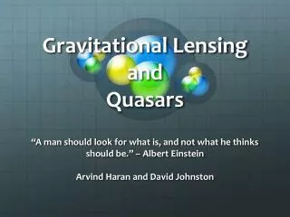
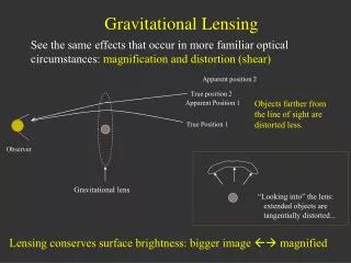
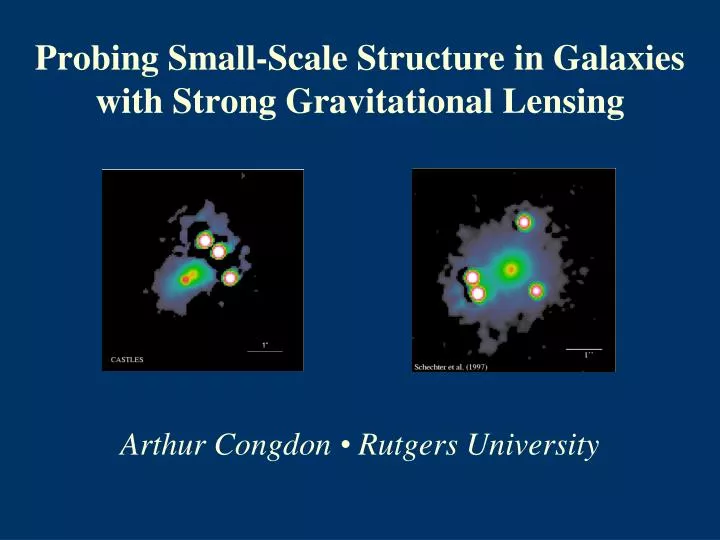
Probing Small-Scale Structure in Galaxies with Strong Gravitational Lensing. Arthur Congdon • Rutgers University. Strong Gravitational Lensing. S. quasar, z ~ 1 - 5. . L. O. galaxy, z ~ 0.2 - 1. Lens equation:. where.

E N D
Probing Small-Scale Structure in Galaxies with Strong Gravitational Lensing Arthur Congdon • Rutgers University
Strong Gravitational Lensing S quasar,z ~ 1-5 L O galaxy, z ~ 0.2-1 Lens equation: where Lensing is sensitive to all mass, be itluminous or dark, smooth or lumpy
Lensing by a Singular Isothermal Sphere (SIS) • Reduced deflection angle: • Lens equation: • Source directly behind lens producesEinstein ringwith angular “radius” qE
SIS Lensing Courtesy of S.Rappaport
SIS with Shear • Lens equation: • 1, 2 or 4 images can be produced
SIS with Shear Courtesy of S.Rappaport
“Double” Lensing by Galaxies:Hubble Space Telescope Images “Quad” “Ring” CASTLES ~ www.cfa.harvard.edu/castles
Quasars as Lensed Sources • Radio emission comes from extended jets • Optical, UV and X-ray emission comes mainly from the central accretion disk
Via Lactea CDM simulation (Diemand et al. 2007)
Via Lactea CDM simulation (Diemand et al. 2007) • Hierarchical structure formation:small objects form first, then aggregate into larger objects
Via Lactea CDM simulation (Diemand et al. 2007) • Hierarchical structure formation:small objects form first, then aggregate into larger objects • Large halos contain the remnants of their many progenitors - substructure
cluster of galaxies,~1015 Msun vs. Clusters look like this - good! single galaxy,~1012 Msun (Moore et al. 1999)
cluster of galaxies,~1015 Msun vs. Galaxies don’t - bad? single galaxy,~1012 Msun (Moore et al. 1999)
Missing Satellites Problem Strigari et al (2007)
Multipole Models of Four-Image Gravitational Lenses with Anomalous Flux Ratios MNRAS 364:1459 (2005)
Four-Image Lenses Source plane Image plane
Universal Relations for Folds and Cusps • Flux relation for a fold pair (Keeton et al. 2005): • Flux relation for a cusp triplet (Keeton et al. 2003): • Valid for all smooth mass models • Deviations small-scale structure
Flux Ratio Anomalies • Many lenses require small-scale structure(Mao & Schneider 1998; Keeton, Gaudi & Petters 2003, 2005) • Could be CDM substructure(Metcalf & Madau 2001; Chiba 2002) • Fitting the lenses requires(Dalal & Kochanek 2002) • Broadly consistent with CDM • Is substructure the only viable explanation?
“Minimum Wiggle” Model • Allow many multipoles, up to mode kmax • Models underconstrained large solution space • Minimize departures from elliptical symmetry. B2045+265
Multipole Formalism • • Convergence: • • Lens potential: • • 2-D Poisson equation: • Fourier expansion:
Observational Constraints • Lens equation: • Image positions give 2n constraints • Magnification: • Flux ratios give n-1 constraints • Combine 3n-1 constraints into a single matrix equation:
Solving for Unknowns • Use SVD to solve for parameters when kmax>4: • Minimize departure from elliptical symmetry (i.e., minimize wiggles): • Adding shear leads to nonlinear equations
Solution for B2045+265 Isodensity contours (solid) and critical curves (dashed)
What Have We Learned from Multipoles? • Multipole models with shear cannot explain anomalous flux ratios • Isodensity contours remain wiggly, regardless of truncation order • Wiggles are most prominent near image positions; implies small-scale structure • Ruled out a broad class of alternatives to CDM substructure
Analytic Relations for Magnifications and Time Delays in Gravitational Lenses withFold and Cusp Configurations Submitted to J. Math. Phys.
Lens TimeDelays Robust probe of dark matter substructure? Q0957+561 Kundićet al. (1997)
Local Coordinates Caustic (source plane) Critical curve (image plane) fold cusp
Perturbation Theory for Fold Lenses Lens Potential: • Lens Equation: • For small displacements: (u1, u2) (eu1, eu2)
Expand image positions in ε: Solve for coefficients to find: Image separation:
Time-Delay Relation for Fold Pairs Scaled Time Delay: Use perturbation theory to get differential time delay: Time-delay anomalies may provide a more sensitive probe of small-scale structure than flux-ratio anomalies
Comparison to “Exact” Numerical Solution Analytic scaling is astrophysically relevant (qE) (qE)
Using Differential Time Delays to Identify Gravitational Lenses with Small-Scale Structure In preparation for submission to ApJ
Dependence of Time Delay on Lens Potential and Position along Caustic • Use h as proxy for time delay • Model lens galaxy as SIE with shear • Higher-order multipoles are not so important here
Time Delays for aRealistic Lens Population • Perform Monte Carlo simulations: • use galaxies with distribution of ellipticity, octopole moment and shear • use random source positions to create mock four-image lenses • use Gravlens software (Keeton 2001) to obtain image positions and time delays • create time delay histogram for each image pair
Histograms for Scaled Time Delay: Folds PG 1115+080 SDSS J1004+4112
Histograms for Scaled Time Delay: Cusps RX J0911+0551 RX J1131-1231
Histograms for Time Delay Ratios: Folds HE 0230-2130 B1608+656
What Have We Learned from Time Delay Analytics and Numerics? • Time delay of the close pair in a fold lens scales with the cube of image separation • Time delay is sensitive to ellipticity and shear, but not higher-order multipoles • For a given image separation and lens potential, the time delay remains constant if the source is not near a cusp • Monte Carlo simulations reveal strong time-delay anomalies in RX J0911+0551 and RX J1131-1231
Acknowledgments I would like to thank my collaborators, Chuck Keeton and Erik Nordgren