Download

1 / 27
280 likes | 558 Vues
Normal Distribution. Introduction. Probability Density Functions. Probability Density Functions…. Unlike a discrete random variable which we studied in Chapter 7, a continuous random variable is one that can assume an uncountable number of values.

E N D
Normal Distribution Introduction
Probability Density Functions… • Unlike a discrete random variable which we studied in Chapter 7, a continuous random variable is one that can assume an uncountable number of values. • We cannot list the possible values because there is an infinite number of them. • Because there is an infinite number of values, the probability of each individual value is virtually 0.
Point Probabilities are Zero • Because there is an infinite number of values, the probability of each individual value is virtually 0. Thus, we can determine the probability of a range of values only. • E.g. with a discrete random variable like tossing a die, it is meaningful to talk about P(X=5), say. • In a continuous setting (e.g. with time as a random variable), the probability the random variable of interest, say task length, takes exactly 5 minutes is infinitesimally small, hence P(X=5) = 0. • It is meaningful to talk about P(X ≤ 5).
Probability Density Function… • A function f(x) is called a probability density function (over the range a ≤ x ≤ b if it meets the following requirements: • f(x) ≥ 0 for all x between a and b, and • The total area under the curve between a and b is 1.0 f(x) area=1 a b x
Uniform Distribution… • Consider the uniform probability distribution (sometimes called the rectangular probability distribution). • It is described by the function: f(x) a b x area = width x height = (b – a) x = 1
Example • The amount of petrol sold daily at a service station is uniformly distributed with a minimum of 2,000 litres and a maximum of 5,000 litres. • What is the probability that the service station will sell at least 4,000 litres? • Algebraically: what is P(X ≥ 4,000) ? • P(X ≥ 4,000) = (5,000 – 4,000) x (1/3000) = .3333 f(x) 2,000 5,000 x
Conditions for use of the Normal Distribution • The data must be continuous (or we can use a continuity correction to approximate the Normal) • The parameters must be established from a large number of trials
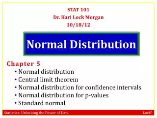
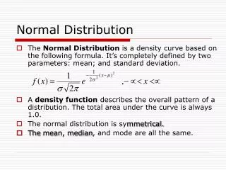
The Normal Distribution… • The normal distribution is the most important of all probability distributions. The probability density function of a normal random variable is given by: • It looks like this: • Bell shaped, • Symmetrical around the mean …
The Normal Distribution… • Important things to note: The normal distribution is fully defined by two parameters: its standard deviation andmean The normal distribution is bell shaped and symmetrical about the mean Unlike the range of the uniform distribution (a ≤ x ≤ b) Normal distributions range from minus infinity to plus infinity
0 1 1 Standard Normal Distribution… • A normal distribution whose mean is zero and standard deviation is one is called the standard normal distribution. • Any normal distribution can be converted to a standard normal distribution with simple algebra. This makes calculations much easier.
Normal Distribution… • Increasing the mean shifts the curve to the right…
Normal Distribution… • Increasing the standard deviation “flattens” the curve…
Calculating Normal Probabilities… • Example: The time required to build a computer is normally distributed with a mean of 50 minutes and a standard deviation of 10 minutes: • What is the probability that a computer is assembled in a time between 45 and 60 minutes? • Algebraically speaking, what is P(45 < X < 60) ? 0
Calculating Normal Probabilities… …mean of 50 minutes and a standard deviation of 10 minutes… • P(45 < X < 60) ? 0
DistinguishingFeatures • The mean ± 1 standard deviation covers 66.7% of the area under the curve • The mean ± 2 standard deviation covers 95% of the area under the curve • The mean ± 3 standard deviation covers 99.7% of the area under the curve Tripthi M. Mathew, MD, MPH
68% of the data 95% of the data 99.7% of the data 68-95-99.7 Rule
Are my data “normal”? • Not all continuous random variables are normally distributed!! • It is important to evaluate how well the data are approximated by a normal distribution
Are my data normally distributed? • Look at the histogram! Does it appear bell shaped? • Compute descriptive summary measures—are mean, median, and mode similar? • Do 2/3 of observations lie within 1 stddev of the mean? Do 95% of observations lie within 2 stddev of the mean?
Law of Large Numbers • Rest of course will be about using data statistics (x and s2) to estimate parameters of random variables ( and 2) • Law of Large Numbers: as the size of our data sample increases, the mean x of the observed data variable approaches the mean of the population • If our sample is large enough, we can be confident that our sample mean is a good estimate of the population mean! Stat 111 - Lecture 7 - Normal Distribution
Points of note: • Total area = 1 • Only have a probability from width • For an infinite number of z scores each point has a probability of 0 (for the single point) • Typically negative values are not reported • Symmetrical, therefore area below negative value = Area above its positive value • Always draw a sketch!