Download
1 / 37
370 likes | 446 Vues
High Throughput Target Identification Stan Young, NISS Doug Hawkins, U Minnesota Christophe Lambert, Golden Helix Machine Learning, Statistics, and Discovery 25 June 03. Micro Array Literature. Guilt by Association : You are known by the company you keep. Data Matrix

E N D
High Throughput Target Identification Stan Young, NISS Doug Hawkins, U Minnesota Christophe Lambert, Golden HelixMachine Learning, Statistics, and Discovery25 June 03
Guilt by Association : You are known by the company you keep.
Data Matrix Goal: Associations over the genes. Genes Tissues Guilty Gene
Goals • Associations. • Deep associations • – beyond 1st level correlations. • 3. Uncover multiple mechanisms.
Problems • n < < p • Strong correlations. • Missing values. • Non-normal distributions. • Outliers. • Multiple testing.
Technical Approach • Recursive partitioning. • Resampling-based, adjusted p-values. • Multiple trees.
Recursive Partitioning • Tasks • Create classes. • How to split. • How to stop.
Recursive Partitioning Top-down analysis Can use any type of descriptor. Uses biological activities to determine which features matter. Produces a classification tree for interpretation and prediction. Big N is not a problem! Missing values are ok. Multiple trees, big p is ok. Clustering Often bottom-up Uses “gestalt” matching. Requires an external method for determining the right feature set. Difficult to interpret or use for prediction. Big N is a severe problem!! Differences:
Forming Classes, Categories, Groups ProfessionAv. Income Baseball Players 1.5M Football Players 1.2M Doctors .8M Dentists .5M Lawyers .23M Professors .09M . . . . .
Forming Classes from “Continuous” Descriptor How many “cuts” and where to make them?
rP = 2.03E-70 aP = 1.30E-66 Signal 2.60 - 0.29 t = = = 18.68 Noise 0.734 1 1 36 1614 + Splitting : t-test n = 1650 ave = 0.34 sd = 0.81 TT: NN-CC n = 1614 ave = 0.29 sd = 0.73 n = 36 ave = 2.60 sd = 0.9
Signal Among Var S(Xi. - X..)2/df1 F = = = Noise Within Var S(Xij - Xi.)2/df2 Splitting : F-test n = 1650 ave = 0.34 sd = 0.81 n = 61 ave = 1.29 sd = 0.83 n = 1553 ave = 0.21 sd = 0.73 n = 36 ave = 2.60 sd = 0.9
How to Stop Examine each current terminal node. Stop if no variable/class has a significant split, multiplicity adjusted.
Levels of Multiple Testing • Raw p-value. • Adjust for class formation, segmentation. • Adjust for multiple predictors. • Adjust for multiple splits in the tree. • Adjust for multiple trees.
Understanding observations Multiple Mechanisms Conditionally important descriptors. NB: Splitting variables govern the process, linked to response variable.
Reality: Example Data 60 Tissues 1453 Genes Gene 510 is the “guilty” gene, the Y.
Split Selection 14 spliters with adjusted p-value < 0.05
Histogram Non-normal, hence resampling p-values make sense.
Single Tree RP Drawbacks • Data greedy. • Only one view of the data. May miss other mechanisms. • Highly correlated variables may be obscured. • Higher order interactions may be masked. • No formal mechanisms for follow-up experimental design. • Disposition of outliers is difficult.
How do you get multiple trees? • Bootstrap the sample, one tree per sample. • Randomize over valid splitters. Etc.
Conclusion for Gene G510 If G518 < -0.56 and G790 < -1.46 then G510 = 1.10 +/- 0.30
Using Multiple Trees to Understand variables • Which variables matter? • How to rank variables in importance. • Correlations. • Synergistic variables.
CorrelationInteractionMatrix Red=Syn.
Summary • Review recursive partitioning. • Demonstrated multiple tree RP’s capabilities • Find associated genes • Group correlated predictors (genes) • Synergistic predictors (genes that predict together) • Used to understand a complex data set.
Needed research • Real data sets with known answers. • Benchmarking. • Linking to gene annotations. • Scale (1,000*10,000). • Multiple testing in complex data sets. • Good visualization methods. • Outlier detection for large data sets. • Missing values. (see NISS paper 123)
Teams U Waterloo : Will Welch Hugh Chipman Marcia Wang Yan Yuan NC State University : Jacqueline Hughes-Oliver Katja Rimlinger U. Minnesota : Douglas Hawkins NISS : Alan Karr (Consider post docs) GSK : Lei Zhu Ray Lam
References/Contact • www.goldenhelix.com. • www.recursive-partitioning.com. • www.niss.org, papers 122 and 123. • young@niss.org • GSK patent.