Download
1 / 10
110 likes | 287 Vues
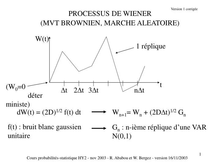
PROCESSUS DE WIENER (MVT BROWNIEN, MARCHE ALEATOIRE). W(t). 1 réplique. t. (W 0 =0 déterministe). t. 2t. 3t. nt. dW(t) = (2D ) 1/2 f(t) dt. W n+1 = W n + (2D t) 1/2 G n. f(t) : bruit blanc gaussien unitaire. G n : n-ième réplique d’une VAR N(0,1).

E N D
PROCESSUS DE WIENER (MVT BROWNIEN, MARCHE ALEATOIRE) W(t) 1 réplique t (W0=0 déterministe) t 2t 3t nt dW(t) = (2D)1/2f(t) dt Wn+1= Wn + (2Dt)1/2 Gn f(t) : bruit blanc gaussien unitaire Gn : n-ième réplique d’une VAR N(0,1) Cours probabilités-statistique HY2 - nov 2003 - R. Ababou et W. Bergez - version 16/11/2003
INTENSITE DU BRUIT BLANC ET COEFFICIENT DE DIFFUSION dW(t) = (2D)1/2f(t) dt D : coefficient de diffusion [m]2[s]-1 f(t) : bruit blanc gaussien d’intensité 1 dW(t) = b(t) dt b(t) = (2D)1/2f(t) b(t) : bruit blanc gaussien d’intensité c [m]2[s]-1avec : c = 2D preuve : Cbb ()= c () = 2D Cff () = 2D () Cours probabilités-statistique HY2 - nov 2003 - R. Ababou et W. Bergez - version 16/11/2003
MOMENTS DU PROCESSUS DE WIENER ESPERANCE E(W(t)) = E(W(0)) = W0 = 0 E(Wn+1) = E(Wn)+ (2Dt)1/2 E(Gn) = … = E(W0) = W0 = 0 VARIANCE DES INCREMENTS E((W(t+)-W(t))2) = 2D || E((Wn+1-Wn)2) = 2Dt E(Gn2) = 2Dt E((Wn+p-Wn)2) = 2D(pt) E(Gn2) = 2D(tn+p - tn) (INCREMENTS STATIONNAIRES) Cours probabilités-statistique HY2 - nov 2003 - R. Ababou et W. Bergez - version 16/11/2003
SIMULATION D ’UN PROCESSUS DE WIENER (estimateur de la variance des incréments : V(=jt) = (N-j)-1 0N-j (Wn+j - Wn )2 Cours probabilités-statistique HY2 - nov 2003 - R. Ababou et W. Bergez - version 16/11/2003
Cours probabilités-statistique HY2 - nov 2003 - R. Ababou et W. Bergez - version 16/11/2003
PROCESSUS DE LANGEVIN dL(t)/dt + 0 L(t) = 0 f(t) avec L(0)=0 (déterministe) f(t) : bruit blanc gaussien unitaire Cff()=() [f]=[s]-1/2 02 : intensité du b. blanc non unitaire b(t)= 0 f(t), [02]=[L]2[s]-1 0 : constante déterministe (résistance visqueuse), [0]=[s]-1 L(t) est un processus non-stationnaire aux temps courts, mais il tend asymptotiquement (pour t >> 1/0 = 0) vers un processus stationnaire de moyenne nulle et d’autocovariance exponentielle : CLL(t,t+)=L2 exp(- 0 ||) 0 = 1/0 est le temps d ’autocorrélation du processus L(t) L2 = 02 /(2 0) est la variance de L(t). Cours probabilités-statistique HY2 - nov 2003 - R. Ababou et W. Bergez - version 16/11/2003
SIMULATION D ’UN PROCESSUS DE LANGEVIN Cours probabilités-statistique HY2 - nov 2003 - R. Ababou et W. Bergez - version 16/11/2003
EQUATION DIFFÉRENTIELLE STOCHASTIQUE ET DISPERSION : • "LÂCHER DE BALLONS GONFLABLES AU STADE TOULOUSAIN" dW/dt + o W = - g + o f(t) , W(0) = W0 V W=mV(t) m : déterministe (éventuellement aléatoire) -g : poussée d ’Archimède volume : déterministe (éventuellement aléatoire) o : coefficient de traînée (Stokes), déterministe f(t) : bruit blanc gaussien unitaire (turbulence) o: amplitude des fluctuations de la force turbulente - g -o W g z Cours probabilités-statistique HY2 - nov 2003 - R. Ababou et W. Bergez - version 16/11/2003
RESULTATS : MOMENTS DE LA VITESSE Hypothèses : V(0)=0, Z(0)=0, m, eto déterministes Notation : Vs = g/(mo) , vitesse de Stokes 0=0/m Equation de la vitesse : dV/dt + oV = - oVS + 0 f(t) t E(V(t))= Vs (1-exp(-ot)) Vs t E(v(t)2)= 02 (1-exp(-ot))/(2o) c2 /2o CVV(t’,t’’) = E(v(t’)v(t’’)) = 02 exp[-o (t’+t’’)] (exp[2omin(t’,t’’)]-1)/(2o) t 0 2 exp[-o |t’-t’’|] /(2o) LA VITESSE TEND VERS UN PROCESSUS STATIONNAIRE Cours probabilités-statistique HY2 - nov 2003 - R. Ababou et W. Bergez - version 16/11/2003
RESULTATS : MOMENTS DE LA POSITION Hypothèses : V(0)=0, Z(0)=0, m, eto déterministes Notation : Vs = g/(mo) , vitesse de Stokes 0 =0/m t Vs (t -1/o) E(Z(t))= Vs (t-(1-exp(-ot))/o) t E(z(t)2) (0/o)2 t = 2 D t C’EST DONC LA VARIANCE D’UN PHENOMENE DE DIFFUSION DU TYPE PROCESSUS DE WIENER (MVT BROWNIEN, MARCHE ALEATOIRE) AVEC UN COEFFICIENT DE DIFFUSION : D = 0.5 (0/o)2 Cours probabilités-statistique HY2 - nov 2003 - R. Ababou et W. Bergez - version 16/11/2003