Download
1 / 21
220 likes | 596 Vues
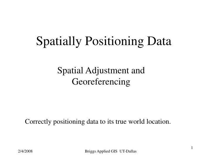
Spatially Positioning Data . Spatial Adjustment and Georeferencing. Correctly positioning data to its true world location. Types. Spatial Adjustment (Transformation) of Vector data Via Spatial Adjustment toolbar See ESRI ArcGIS 9: Editing in ArcMap , Chapter 8, Spatial Adjustment

E N D
Spatially Positioning Data Spatial Adjustment and Georeferencing Correctly positioning data to its true world location. Briggs Applied GIS UT-Dallas
Types • Spatial Adjustment (Transformation) of Vector data • Via Spatial Adjustment toolbar • See ESRI ArcGIS 9:Editing in ArcMap, Chapter 8, Spatial Adjustment • Georeferencing of an Image (Raster data) • Via Georeferencing toolbar • Typically used for: • satellite images • aerial photographs • scanned CAD drawings • Positioning a vector CAD file • Via Georeferencing Toolbar in ArcGISG 9.2, or via Properties/Transformation in ArcGIS 9.1 • Is planimetrically accurate to start with (or should be) • Only requires translation of origin and scale change Briggs Applied GIS UT-Dallas
Spatial Adjustment Capabilities Spatial Adjustment Toolbar provides three spatial adjustment capabilities: • Repositioning of a source vector layer to correspond with a correctly positioning target layer (which may be vector or raster) • Via Homogeneous transformations (overlay) • Can select among Affine, Similarity, or Projective transforms • Via Differential Transformation (overlay) • Rubber sheeting using a TIN-like (set of triangles) structure • Edge Matching (side-by-side) • Use Edge Snapping of features at map edges to align two adjacent data sets (map sheets) • Attribute Transfer (non-spatial attributes) • Transfer of non-spatial attributes from a feature in one layer to a feature in another layer • Intended for Conflation applications Displacement links Adjustment area Links Table
Implementing a Spatial Transformation Essentially involves five steps • Open the layer’s folder or gdb for editing on Editor toolbar • Select the layer to be transformed on Spatial Transformation toolbar • Create Displacement Links which link source coordinates to destination coordinates -- several ways to do this (see following slides) • Select a Transformation Method -- several choices (see following slides for detail) • Perform the actual transformation and save results Warnings: --be sure that the coordinate system of the data frame has been defined before you start --always insert a new data frame or open a new map document for each layer you wish to transform --start a new map document if you wish to use the transformed layer in a layout Briggs Applied GIS UT-Dallas
Creating Displacement Links for Vector • displacement links define the source and destination coordinates for the adjustment. • Links are represented as arrows with the arrowhead pointing towards the destination location. • They are stored in the displacement links table (click to open) • Displacement links can be created: • Interactively one at a time using the displacement link tool • Must click source (file to be moved) first, then destination • Can adjust an existing link with the modify link tool • Can “lock” a location so it does not move using identity link tool • Can limit adjustment to a specific area • By reading in a link file (tab delimited text format) containing two sets of X,Y coordinates (four columns) for source and destination (may also contain an initial column with Ids, for a total of five columns) • Created in Excel or other editing program • Saved from the displacement links table in a previous adjustment session • By reading in a control file (tab delimited text format) containing one set of X,Y coordinates (two columns) of control points for destinations • Derived from GPS for example Go to Help/Spatial Adjustment for Editing in ArcMap for details
The affine transformation function is: • x’ = Ax + By + Cy’ = Dx + Ey + F • where x and y are coordinates of the input layer and x’ and y’ are the transformed coordinates. • The C and F parameters control shift in origin (translation) • A, B, D, E control scale and rotation • their values are determined by comparing the location of source and destination control points. • Scales, skews, rotates, and translates • 6 unknowns( A,B,C,D,E,F) so a minimum of three “displacement links” required • Usually estimated via statistical techniques which minimize RMSE • this requires four links minimum but more usually used to “average the error” • Little benefit from more than 18-30 links • The most common choice Transformation types: Affine Briggs Applied GIS UT-Dallas
Transformation types: Similarity or Conformal The similarity transform function is: x’ = Ax + By + C y’ = -Bx + Ay + F where: • A = s · cos tB = s · sin tC = translation in x directionF = translation in y direction and: • s = scale change (same in x and y directions)t = rotation angle, measured counter-clockwise from the x-axis • Scales, rotates, and translates the data • Does not independently scale the axes, nor introduce any skew. • It maintains the aspect ratio of the features transformed (e.g. squares remain squares) • Four unknowns (A,B,C,F) thus requires a minimum of two displacement links X X Briggs Applied GIS UT-Dallas
Transformation types: Projective • based upon a more complex formula x’ = (Ax + By + C) / (Gx + Hy + 1)y’ = (Dx + Ey + F) / (Gx + Hy + 1) • used to transform data captured directly from aerial photography. • requires a minimum of four displacement links. • For information see: Moffitt, F.H. and E.M. Mikhail. Photogrammetry. Third Edition. Harper & Row, Inc., 1980. Slama, C.C., C. Theurer, and S.W. Henriksen (eds.). Manual of Photogrammetry. 4th Edition. Chapter XIV, pp. 729-731. ASPRS, 1980. Briggs Applied GIS UT-Dallas
Rubbersheeting in Spatial Transformations “Uneven” Geometric distortions commonly occur in source data. • imperfect registration in map compilation, • lack of geodetic control in source data, • Rubbersheeting corrects flaws through the geometric adjustment of coordinates through a differential transformation • The source layer is adjusted to the more accurate target layer. • surface is literally stretched, moving features using a piecewise transformation that preserves straight lines. • Two types of processing: Natural Neighbor and Linear Target layer (accurate) Source layer (inaccurate)
How Rubber Sheeting Works for Spatial Transformations • Two temporary TIN-like structures are created for source (from) and target (to) layers using Thiessen Polygons/Delauney triangles constructed from the control points (displacement links) • Each corner of triangle has X,Y,Z coordinates • The z value in the source (from) layer codes the amount of adjustment (rather than “elevation as in standard TIN) • Since adjustment is known at each corner of triangle it can then be interpolated for all other points • Two interpolation methods used • Linear, quick and accurate if you have lots of displacement points over the area being adjusted, but doesn’t take into account “the neighborhood” • Natural neighbor (similar to IDW--inverse distance weighting), slower but more accurate if you don’t have many displacement links Briggs Applied GIS UT-Dallas
Source (less accurate) Target (more accurate) Edge Matching • aligns features along the edge of one layer to features of an adjoining layer. • The layer with the less accurate features is adjusted, while the adjoining layer is used as the control. Briggs Applied GIS UT-Dallas
Attribute Transfer and Conflation • Attribute transfer is typically used to copy attributes from a less accurate layer to a more accurate one. • Conflation: “thecreation of a new master coverage from quality spatial data in one source and quality attribute data in another,” • For example, it can be used to transfer the names of hydrological features from a previously digitized and highly generalized 1:500,000 scale map to a more detailed and positionally accurate 1:24,000 scale • To transfer street names from a TIGER-derived file to a line layer digitized from positionally accurate digital orthos • you can specify which attributes to transfer between layers, then interactively choose the source and target features. • Typically, Rubbersheeting is used first to align the layers spatially then Attribute Transfer is used to transfer the attributes • In practice, I’ve often found it easier to do it in the reverse order! • if layers too close, difficult to establish the link necessary for the attribute transfer. • Attribute transfer tool is not as useful as might appear because it’s feature by feature • only really helps if have multiple attributes to transfer • An alternative is to do a Rubbersheeting first, the use a Spatial Join to accomplish a “batch transfer” for multiple features simultaneously Briggs Applied GIS UT-Dallas
Open Links table Create control point links (displacement links) Use to help “Fit image to display” Use to start all over again Georeferencing • Used for positioning rasters and vector CAD data in ArcGIS 9.2 • Yes, this is an “odd couple” • CAD is a vector data set type! • Implemented via the Georeferencing toolbar • Use for scanned maps, scanned CAD drawings, photographs, satellite images, etc. in standard image formats such as .jpg, .gif, .tif • Raster data sets in GRID, ERDAS IMAGINE, etc format • CAD vector data sets in .dxf (AutoCAD) ,dwg (AutoCAD) and .dgn (Microstation) format Briggs Applied GIS UT-Dallas
Types of transformations for Georeferencing Rasters and Images • 1st order polynomial (affine) • requires a minimum of 3 displacement links, but should have more even though 3 gives RMSE=0! • is a homogeneous transformation: only shifts origin, scales and rotates • straight lines will be preserved • 2nd order polynomial • requires 6 points (displacement links) minimum • is a differential transformation so it “warps” the raster • straightlines on raster may no longer be straight • 3rd order polynomial • requires 10 points minimum Polynomials are global transformations which strive to achieve a best fit globally or overall. Only 1st order with exactly 3 points will exactly match control points. Briggs Applied GIS UT-Dallas
Types of transformations for Georeferencing Rasters and Images--continued 4. Spline transformation • Often referred to as a “rubbersheeting” transformation • optimizes for local accuracy but not global accuracy. • control points exactly match to target control points • useful when the control points are very important and must be registered precisely. • requires a minimum of three control points 5. Adjust transformation • optimizes for both global Least Squares Fit and local accuracy. • Uses an algorithm that combines a polynomial transformation and TIN interpolation techniques. • requires a minimum of three control points. All transformation types are selected by going to: Georeferencing/Transformation Briggs Applied GIS UT-Dallas
rmse = e12 + e22 + e32 +...+ en2 n-1 Comments on Polynomials and Goodness of Fit • Example equation for second degree polynomial for the X coordinate transformation: X’ = b1+b2X+b3Y+b4X2+b5Y2+b6XY • Since there are six unknowns, a minimum of 6 displacement points is required • Higher order polynomials provide more flexibility for warping the surface to fit the control points, however • More displacement points are required • They can significantly deform the non-control point coordinates and produce significant distortions—be careful! • RMSE (root mean square error) can be used to assess “goodness of fit” to control points but this does not measure the non-control point distortion • ESRI calls this LSF-least squares fit. • RMSE is only comparable within a given polynomial level • It automatically goes down as higher order polynomials are used where ei is the distance between the source control point iafter transformation and the target control point i Briggs Applied GIS UT-Dallas
Saving Georeferencing Results • Update Georeferencing • Adds world file only, which contains transformation parameters for rasters • Image file unchanged • Rectify • Rewrites image file • Use if need to do spatial analysis on file, in which case choose GRID as output type • Can save output as JP2, JPG, GIF, GRID, ERDAS IMAGINE, TIFF or BMP • New square output cells created, so issue arises how the raster values are assigned from input to output cells since the source will have been “warped” • Nearest neighbor takes the value from the cell closest to the transformed cell. It’s the fastest. Should always be used for categorical data since it preserves original values (a 3 will never become 3.25). • Bilinear interpolation takes average of values for four nearest cells in the untransformed data weighted by distance to the transformed cell location. Use only for continuous data such as elevation, slope. • Bilinear smooths data like a low pass filter. • Cubic convolution takes average of values for 16 nearest cells in the untransformed data weighted by distance to the transformed cell location. Again, use only for continuous data. Commonly used for photographs and similar data. • Cubic tends to sharpen data like a high pass filter.
World File for Raster data--not the same as for CAD--contains affine equation parameters Equation for Affine transformation World file for Parameters raster data 1.60000002384186 - A 0.00000000000000 - D 0.00000000000000 - B -1.60000002384186 - E 2496000.75 - C 7049998.50 - F (for UTD image: 24967042.jgw) x1 = Ax + By + C y1 = Dx + Ey + F The y-scale (E) is negative because the origin of an image is located in the upper left corner, whereas the origin of the map coordinate system is located in the lower left corner. Row values in the image increase from the origin downward, while y-coordinate values in the map increase from the origin upward. (See ArcHelp) Briggs Applied GIS UT-Dallas
Positioning CAD files--concept • A CAD layer is planimetrically accurate at start (or should be!) • Planimetric: map accurate in two dimensions • Only requires translation of origin, and homogeneous scale change (same change on both X and Y axes) • Equivalent to a similarity transformation which is conformal and preserves all local angles • Based on identifying only two common points • Thus, transformation is solved mathematically rather than statistically • Thus assumes there is no error in the data Briggs Applied GIS UT-Dallas
Positioning CAD Files--Implementation In ArcGIS 9.2 and later • Use Georeferencing toolbar to obtain two control point pairs (displacement links) only • Methodology same as for georeferencing raster file • Any of the CAD feature class layers may be used--the transformation is applied to all • A CAD world file is created when you click Update Georeferencing • Named the same as the CAD file, with extension .wld • Note: CAD world file differs from JPEG or TIFF world file! • Contains X,Y control point pair coordinates, not transformation parameters Note: heading not included in file XCAD Source YCAD Source XREAL Map YREAL Map 240.000000, 750.500000 2505108.552674, 7046646.373472 4134.000000, 2550.000000 2505523.148640, 7046837.967062 Briggs Applied GIS UT-Dallas
Positioning CAD Files--Implementation In ArcGIS 9.1 and earlier • Must have, a priori, X,Y coordinates for two pairs of corrresponding points in the CAD and the real world • Points may be entered: • via the Properties/Transformations tab of the CAD layer itself (not available in ArcGIS 9.2) • By creating a CAD world file containing corresponding XY coordinate pairs • Named the same as the CAD file, with extension .wld • Note: CAD world file differs from JPEG or TIFF world file! Note: heading not included in file XCAD Source YCAD Source XREAL Map YREAL Map 240.000000, 750.500000 2505108.552674, 7046646.373472 4134.000000, 2550.000000 2505523.148640, 7046837.967062 Briggs Applied GIS UT-Dallas