Download
1 / 77
790 likes | 1.18k Vues
Concept of Routing in Network Layer. Network Layer II (routing). Routing Styles: Static vs. Dynamic Routing Routing Protocols/Algorithms Routing Table Routing Information Protocol (RIP) & Distance Vector Routing (DVR) Open Shortest Path First (OSPF) & Link State Routing (LSR)

E N D
Concept of Routing in Network Layer
Network Layer II (routing) • Routing Styles: • Static vs. Dynamic Routing • Routing Protocols/Algorithms • Routing Table • Routing Information Protocol (RIP) & Distance Vector Routing (DVR) • Open Shortest Path First (OSPF) & Link State Routing (LSR) • Dijkstra’s “Shortest Path” Algorithm • Border Gateway Protocol (BGP) and Path Vector Routing (PVR)
Routing Protocol & Routing Algorithm • A Routing Protocol is a combination of rules and procedures that lets routers in an internet inform each other of changes. It allows routers to share whatever they know about the internet or their neighbourhood. • A Routing Algorithm is that part of network layer software responsible fro deciding which output line and incoming packet should be transmitted on.
Routing • Routing requires a host or a router to have a routing table. • Usually when a host has a packet to send or when a router has received a packet to be forwarded, it looks at this table to find the route to the final destination. • However, this simple solution is impossible in today’s Internet world because the number of entries in the routing table makes the table lookups inefficient. • Need to make the size of table manageable and handles issues such security at the same time. The key question is how to design the routing table. • Next-hop routing, Network-specific routing, host specific routing • Static versus Dynamic Routing • Routing Protocols: RIP, OSPF, BGP • Routing Algorithms: DVR, LSR, PVR
Next-hop routing Next-hop routing holds only the information that leads to the next hop instead of complete route.
Network-specific & host-specific routing The destination host address is given in the routing table; to have greater control over routing. Instead of having an entry for every host connected to the same network, only one entry is needed to defined the address of the network itself. All host connected to the same network as one single entity.
Default routing R1 is used to route packets to hosts connected to N2. However, R2 is used to as default to route other packets to the rest of Internet without listing all the networks involved Only one default routing is allowed with network address 0.0.0.0
General Routing Table Flags U The router is up and running. G The destination is in another network. H Host-specific address. D Added by redirection. M Modified by redirection.
Routing table • Generally, a routing table needs a minimum of 4 columns: mask, destination network address, next hop address and interface. • When a packet arrives, the router applies the mask to the destination address it receives (one-by-one until a match is found) in order to find the corresponding destination network address. • So, the mask serves as essential tool to match destination address in routing table and the address it receives. • If found, the packet is sent out from the corresponding interface in the table. If not found, the packet is delivered to the default interface which carries the packet to default router.
Configuration for routing example MaskDest. Next HopI. 255.0.0.0 111.0.0.0 -- m0 255.255.255.224 193.14.5.160 - m2 255.255.255.224 193.14.5.192 - m1 255.255.255.255 194.17.21.16 111.20.18.14 m0 255.255.255.0 192.16.7.0 111.15.17.32 m0 255.255.255.0 194.17.21.0 111.20.18.14 m0 0.0.0.0 0.0.0.0 111.30.31.18 m0 Standard delivery Host-specific Network-specific Default
Example 1 Router R1 receives 500 packets for destination 192.16.7.14; the algorithm applies the masks row by row to the destination address until a match (with the value in the second column of Dest. in table) is found: Rule of thumb: Apply the individual mask (from Routing table) to the received destination address (row-by-row) and see if its matches any of the DEST address stated in its routing table. If match is found, then stop Solution Direct delivery 192.16.7.14 & 255.0.0.0 192.0.0.0 no match to 111.0.0.0 192.16.7.14 & 255.255.255.224 192.16.7.0no match to 193.14.5.160 192.16.7.14 & 255.255.255.224 192.16.7.0no match to 193.14.5.192 Host-specific 192.16.7.14 & 255.255.255.255192.16.7.14no match to 194.17.21.16 Network-specific 192.16.7.14 & 255.255.255.0192.16.7.0 match to 192.16.7.0
Example 2 Router R1 receives 100 packets for destination 193.14.5.176; the algorithm applies the masks row by row to the destination address until a match is found: Solution Direct delivery 193.14.5.176 & 255.0.0.0 193.0.0.0 no match 193.14.5.176 & 255.255.255.224193.14.5.160 match
Example 3 Router R1 receives 20 packets for destination 200.34.12.34; the algorithm applies the masks row by row to the destination address until a match is found: Solution 200.34.12.34 & 255.0.0.0 200.0.0.0 no match 200.34.12.34 & 255.255.255.224200.34.12.32 no match 200.34.12.34 & 255.255.255.224200.34.12.32 no match 200.34.12.34 & 255.255.255.255200.34.12.34 no match 200.34.12.34 & 255.255.255.0 200.34.12.0 no match 200.34.12.34 & 255.255.255.0 200.34.12.0 no match Default 200.34.12.34 & 0.0.0.0 0.0.0.0. match
Solution MaskDestinationNext HopI. 255.255.0.0 134.18.0.0 -- m0 255.255.0.0 129.8.0.0 222.13.16.40 m1 255.255.255.0 220.3.6.0 222.13.16.40 m1 0.0.0.0 0.0.0.0 134.18.5.2 m0 Example 4 Make the routing table for router R1 in figure below
Subnet maskDestination Next HopI. 255.255.255.0 200.8.4.0 ---- m2 255.255.255.0 80.4.5.0 201.4.10.3 m1 or 200.8.4.12 or m2 255.255.255.0 80.4.6.0 201.4.10.3 m1 or 200.4.8.12 or m2 0.0.0.0 0.0.0.0 m0 Example 5 Make the routing table for router R1 in figure below Solution
Note In classless addressing, we need at least four columns in a routing table.
Routing Tables in IP with CIDR(Classless InterDomain Routing) For each entry in the routing table: MaskedAddress := EntryMask (bitAND) IPDatagramDestinationAddress; if (MaskedAddress == EntryDestination) Mark the entry; Choose the marked entry with the longest Mask prefix.
m3 Make a routing table for router R1, using the configuration in Figure below Example 7a Solution Routing table for router R1 in Figure above The table is sorted from the longest mask to the shortest mask.
Show the forwarding process if a packet arrives at R1 with the destination address 180.70.65.140. Example 7b Solution The router performs the following steps: 1. The first mask (/26) is applied to the destination address. The result is 180.70.65.128, which does not match the corresponding network address. 2. The second mask (/25) is applied to the destination address. The result is 180.70.65.128, which matches the corresponding network address. The next-hop address and the interface number m0 are passed on for further processing.
Show the forwarding process if a packet arrives at R1 with the destination address 201.4.22.35. Example 7c Solution The router performs the following steps: 1. The first mask (/26) is applied to the destination address. The result is 201.4.22.0, which does not match the corresponding network address. 2. The second mask (/25) is applied to the destination address. The result is 201.4.22.0, which does not match the corresponding network address (row 2). 3. The third mask (/24) is applied to the destination address. The result is 201.4.22.0, which matches the corresponding network address..
Show the forwarding process if a packet arrives at R1 with the destination address 18.24.32.78. Example 7d Solution This time all masks are applied, one by one, to the destination address, but no matching network address is found. When it reaches the end of the table, the module gives the default next-hop address 180.70.65.200 (because it could not find the match) . This is probably an outgoing package that needs to be sent, via the default router, to someplace else in the Internet.
Routing/routers • An internet is a combination of networks connected by routers. • When a packet goes from a source to a destination, it will pass through many routers until it reaches the router attached to destination network. • A router consults a routing table when a packet is ready to be forwarded. The routing table specifies the optimum path for the packet and can be either static of dynamic. Dynamic routing is more popular. • Static table does not change frequently. Dynamic table is updated automatically when there is a change somewhere in the network; i.e when a route is down or a better route has been created. • Routing protocols is a combination of rules/procedures that lets routers in the internet inform one another when changes occur; mostly based on sharing/combining information between routers at different networks.
Unicast Routing • Unicast = one source and one destination. (1-to-1 relationship). • In Unicast routing, when a router receives a packet, it forwards the packet thru only one of its ports as defined in the routing table. The router may discard the packet if it cannot find the destination address • Questions: In dynamic routing, how does the router decides to which network should it pass the packet next? What routing algorithm is the routing based on? The decision is based on optimisation: which of the available pathways is the best/optimum path? • But how to measure? A metric is a cost assigned for passing thru a network and the total metric of a particular route is equal to the sum of the metrics of networks that comprise the route. • Simple protocols such as Routing Information Protocol (RIP), treat all network equally; cost of passing each network is the same as one hop count per network. • Other sophisticated protocols e.g. OSPF, based on services required and using different metrics: max throughput, minimum delay.
Routing Protocol: Interior Vs Exterior
Routing Architecture in the Internet Fact: Nobody owns the whole Internet. However, parts of the Internet are owned and administered by commercial and public organisations (such as ISPs, universities, governmental offices, research institutes, companies etc.). • Idea: • Divide the Internet in Autonomous Systems (AS) that are independently administered by individual organisations. • Let each administrative authority use its own routing protocol within the AS. • Let’s use one routing protocol to exchange routing information among AS.
Routing Architecture in the Internet An AS is a group of networks and routers under the authority of a single administrator.
Static versus Dynamic Routing A static routing table contains information entered manually Usually remained unchanged. A dynamic routing table is updated periodically or whenever necessarily using one of the dynamic routing protocols such as RIP, OSPF, or BGP.
Routing Protocols: Interior vs Exterior • Routing inside an AS is referred to as interior routing whereas routing between ASs is referred to as exterior routing. • Each AS can choose one or more interior routing protocols inside an AS. • Only one exterior routing protocol is usually chosen to handle routing between ASs. • To know the next ’path’ (or router) a packet should be pass-on, the decision is based on some optimisation rule/protocol, e.g. using different assignment of the cost (metric) for each passing through a network for different routing Protocol above.
Interior Routing Protocol 1: Routing Information Protocol (RIP)
Distance Vector Routing (DVR) • 3 keys to understand how this algorithm works: • Sharing knowledge about the entire AS. Each router shares its knowledge about the entire AS with neighbours. It sends whatever it has. • Sharing only with immediate neighbours. Each router sends whatever knowledge it has thru all its interface. • Sharing at regular intervals. sends at fixed intervals, e.g. every 30 sec. • Problems: Tedious comparing/updating process, slow response to infinite loop problem, huge list to be maintained!!
Updating in distance vector routing example: C to A From A From C A to A via C: ACA = AC+ CA = 2+2 A to B via C: ACB = AC + CB = 2+4 A to D via C: ACD = AC + CD = 2+ inf. A to E via C: ACD = AC + CE = 2+4 A to C via C: ACC = AC + CC = 2+0
Example-1 Distance Vectors below that are received at node-B in a network. Given the estimated distance to its neighbours: node-A, node-D and node-F are 6, 9, and 11 hops, respectively. Find the new distance vector at B. (Note: The new vector must include the next hop and the estimated cost). 34
A 6 B 9 D 11 F Solution 35
Example-2 Distance Vectors below that are received at node-A in a network. Given that the estimated delay to its neighbours node-B, node-F and node-H are 6, 10, and 8 units, respectively. Find the new distance vector at A. (The new distance vector must indicate the next hop and the estimated delay) 36
B 6 A 8 H 10 F Solution 37
DVR extra example from Tenenbaum (with estimated delay) Neighbour routers Each router maintain a table (a vector) giving the best known metric (or delay) to each destination and which line to use. These tables are then updated by exchanging information with the neighbours (direct link, 1 hop) • A subnet. (b) Input from A, I, H, K, and the new routing table for J. 1st DRAWBACK: VERY SLOW!!!
Routing Information Protocol (RIP) • RIP is based on distance vector routing, which uses the Bellman-Ford algorithm for calculating the routing table. • RIP treats all network equals; the cost of passing thru a network is the same: one hop count per network. • Each router/node maintains a vector (table) of minimum distances to every node. (the least-cost route btw any nodes is the route with the minimum number of hop-count). • The hop-count is the number of networks that a packet encounters to reach its destination. Path costs are based on number of hops. • In distance vector routing, each router periodically shares its knowledge about the entire internet with its neighbour. • Each router keeps a routing table that has one entry for each destination network of which the router is aware. • The entry consists of Destination Network Address/id, Hop-Count and Next-Router.
Example of Initial routing tables (RIP) in a small autonomous system
Infinite loop problem Initially, X was running before the failure and the number of hop count from X is available in each node A and B. After the failure of X, the connection is broken and A changes its table to infinity hop count about X, while B is still preserving the same count. In the subsequent update, if B sends its table before A, then A assumes B has found a way to reach X, while B in turn assumes that A has changed it table and update accordingly. The hop count continues to increase gradually until infinity.
Infinite loop problem in DVR A initially up then down A initially down; hence The count-to-infinity problem! Good news (a) travels faster than bad news (b) React rapidly to good news but slowly to bad news Although it will eventual converge to correct answer, they adapt slowly, they must be told to change. Convergence to the correct answer is slow.
Interior Routing Protocol 2: Open Shortest Path First Protocol (OSPF)
Open Shortest Path First (OSPF) • OSPF uses link state routing to update the routing table in an area; (OSPF divides an AS into different areas). • Unlike RIP, OSPF treats the entire network within differently with different philosophy; depending on the types, cost (metric) and condition of each link: to define the ‘state’ of a link. • OSPF allows the administrator to (only) assign a cost for passing through a network based on the type of service required. e.g. minimum delay, maximum throughput. (but not stating exact path) • Each router should have the exact topology of the AS network (a picture of entire AS network)at every moment. The topology is a graph consisting of nodes and edges. • Each router needs to advertise to the neighbourhood of every other routers involved in an Area. (flood)
Open Shortest Path First (OSPF) Areas in an Autonomous System (AS>Areas) OSPF divides an AS into areas. An area is a collection of network, hosts and routers all contained within an AS. Routers inside an area flood the area with routing info. At the border of an Area, special routers called Area Border routers summarize the info. about the area and send it to other area. Among the areas inside an AS is a special area called the Backbone connecting all areas through Backbone routers and serves as a primary area to the outside (other ASs) via the AS Boundary router.
Link State Routing (LSR) • Like RIP, in link state routing, each router also shares its knowledge about its neighbourhood with every routers in the area. • However, in LSR, the link-state packet (LSP) defines the best known network topology (of an area) is sent to every routers (of other area) after it is constructed locally. Whereas RIP slowly converge to final routing list based information received from immediate neighbours. • 3 keys to understand how this algorithm works: • Sharing knowledge about the neighbourhood. Each router sends the state of its neighbourhood to every other router in the area. • Sharing with every other routers. Thru process of flooding. each router sends the state of its neighbourhood thru all its output ports and each neighbour sends to every other neighbours and so on until all routers received same full information eventually. (DO NOT SEND UPDATE FREQUENTLY) • Sharing when there is a change. Each router share its state of its neighbour only when there is a change; contrasting DVR results in lower traffic.
Link State Routing (LSR) • LSR differs from DVR in the following: • Can use different cost/metric instead of just hop-counts • Routing update is only performed when there is a change in topology or after a long period (every 30 minutes) • Each router has an ‘overall map’ or knowledge of the entire network topology within the AS or an area of the AS • Because the network-topology is known in advanced, routers can work out which is the best route to choose between two nodes if there is more than two alternative routes/paths – by shortest path algorithm. • This solve the problem of infinity-loop as all routers will be informed instantly by LSA and paths are recalculated immediately. • From the received LSPs and knowledge of entire topology, a router can then calculate the shortest path between itself and each network. • Usually works better for large networks. 49
Types of links When the link between two routers is broken, the administrator may create a virtual link between them using longer path that probably goes through several routers