Download
1 / 83
830 likes | 871 Vues
Learn about arrays as a fundamental data structure, including operations, implementation, and advanced algorithms like sorting and searching. Explore array ADT, usage, and analogies for better comprehension. Enhance your programming skills this week!

E N D
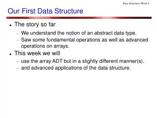
Data Structures Week 3 Our First Data Structure • The story so far • We understand the need for data structures • We have seen a few analysis techniques • This week we will • see a very simple data structure – the array • its uses, details, • and advanced applications of this data structure.
Data Structures Week 3 A Data Structure • How should we view a data structure? • From a implementation point of view • Should implement a set of operations • Should provide a way to store the data in some form. • From a user point of view • should use it as a black box • call the operations provided • Analogy : C programming language has a few built-in data types. • int, char, float, etc.
Data Structures Week 3 Analogy • Consider a built-in data type such as int • A programmer • can store an integer within certain limits • can access the value of the stored integer • can do other operations such add, subtract, multiply, ... • Who is implementing the data structure? • A compiler writer. • Interacts with the system and manages to store the integer.
Data Structures Week 3 An Abstract Data Type • A data structure can thus be looked as an abstract data type. • An abstract data type specifies a set of operations for a user. • The implementor of the abstract data type supports the operations in a suitable manner. • One can thus see the built-in types also as abstract data types.
Data Structures Week 3 The Array as a Data Structure • Suppose you wish to store a collection of like items. • say a collection of integers • Will access any item of the collection. • May or may not know the number of items in the collection. • Example settings: • store the scores on an exam for a set of students. • store the temperature of a city over several days.
Data Structures Week 3 The Array as a Data Structure • In such settings, one can use an array. • An array is a collection of like objects. • Usually denoted by upper case letters such as A, B. • Let us now define this more formally.
Data Structures Week 3 The Array ADT • Typical operations on an array are: • create(name, size) : to create an array data structure, • ElementAt(index, name) : to access the element at a given index i • size(name) : to find the size of the array, and • print(name) : to print the contents of the array • Note that in most languages, elementAt(index, name) is given as the operation name[index].
Data Structures Week 3 The Array Implementation Algorithm Create(int size, string name) begin name = malloc(size*sizeof(int)); end Algorithm Print(string name) begin for i = 1 to n do printf("%d t", name[i]); end-for; end; Algorithm ElementAt(int index, string name) begin return name[i]; end Algorithm size(string name) begin return size; end;
Data Structures Week 3 Further Operations • The above operations are quite fundamental. • Need further operations for most problems. • We will now see some such operations.
Data Structures Week 3 The above is an iterative way to find the minimum element of a given array. Recall that we attempted a recursive version earlier. Minimum and Maximum Algorithm FindMinimum(name) begin int min,i; min = name[1]; for i = 2 to n do if min > name[i] then min = name[i]; end-for; end;
Data Structures Week 3 Minimum and Maximum • Notice that the algorithm makes n − 1 iterations of the loop and hence makes n − 1 comparisons. • A similar approach also works for finding the maximum. • What if we want to find both the maximum and the minimum together? • Can we do it in less than 2n comparisons?
Data Structures Week 3 Minimum and Maximum Algorithm MinimumMaximum(name) begin int max, min; max = name[1], min = name[1]; for i = 1 to n/2 do element1 = name[2i − 1]; element2 = name[2i]; if element1 < element2 then x = element1, y = element2; else x = element2, y = element1; if x < min then min = x; if max < y then max = y; end-for end;
Data Structures Week 3 Maximum and Minimum • How many comparisons does the above algorithm make? • Not just in the asymptotic sense, but actual count.
Data Structures Week 3 Sorting • Sorting is a fundamental concept in Computer Science. • several application and a lot of literature. • We shall see an algorithm for sorting.
Data Structures Week 3 QuickSort • The quick sort algorithm designed by Hoare is a simple yet highly efficient algorithm. • It works as follows: • Start with the given array A of n elements. • Consider a pivot, say A[1]. • Now, partition the elements of A into two arrays AL and AR such that: • the elements in AL are less than A[1] • the elements in AR are greater than A[1]. • Sort AL and AR, recursively.
Data Structures Week 3 How to Partition? • Here is an idea. • Suppose we take each element, compare it with A[1] and then move it to AL or AR accordingly. • Works in O(n) time. • Can write the program easily. • But, recall that space is also an resource. The above approach requires extra space for the arrays AL and AR • A better approach exists.
Algorithm Partition • Algorithm Partition is given above. Procedure Partition(A,n) begin pivot = A(n); less = 0; more = 1; for more = 1 to n do if A(more) < pivot then less++; swap(A(more), A(less)); end swap A[less+1] with A[n]; end
Correctness by Loop Invariants • Example run of Algorithm Partition 12 34 27 19 36 29 10 22 28 12 34 27 19 36 29 20 22 28 12 27 34 19 36 29 20 22 28 12 27 34 19 36 29 20 22 28 12 27 19 34 36 29 20 22 28 12 27 19 34 36 29 20 22 28 12 27 19 34 36 29 20 22 28 12 27 19 20 36 29 34 22 28 12 27 19 20 22 29 34 36 28
The Basic Step in Partition left right n-1 1 n < Pivot > Pivot Pivot
The Basic Step in Partition left right n-1 • The main action in the loop is the comparison of A[k+1] with A[n]. • Consider the case when A[k+1] < A[n]. 1 n < Pivot > Pivot Pivot 1 n < Pivot > Pivot Pivot n-1 left right
The Basic Step in Partition left right n-1 • Consider the case when A[k+1]> A[n] 1 n < Pivot > Pivot Pivot 1 n < Pivot > Pivot Pivot n-1 left right
Another Operation – Prefix Sums • Consider any associative binary operator, such as +, and an array A of elements over which o is applicable. • The prefix operation requires us to compute the array S so that S[i] = A[1]+A[2]+ · · · +A[i]. • The prefix operation is very easy to perform in the standard sequential setting.
Example A = (3, -1, 0, 2, 4, 5) S[1] = 3. S[2] = -1+3 = 2, S[3] = 0 + 2 = 2,... The time taken for this program is O(n). Sequential Algorithm for Prefix Sum Algorithm PrefixSum(A) S[1] = A[1]; for i = 2 to n do S[i] = A[i] + S[i-1] end-for
Our Interest in Prefix • The world is moving towards parallel computing. • This is necessitated by the fact that the present sequential computers cannot meet the computing needs of the current applications. • Already, parallel computers are available with the name of multi-core architectures. • Majority of PCs today are at least dual core.
Our Interest in Prefix • Programming and software has to wake up to this reality and have a rethink on the programming solutions. • The parallel algorithms community has fortunately given a lot of parallel algorithm design techniques and also studied the limits of parallelizability. • How to understand parallelism in computation?
Parallelism in Computation • Think of the sequential computer as a machine that executes jobs or instructions. • With more than one processor, can execute more than one job (instruction) at the same time. • Cannot however execute instructions that are dependent on each other.
Parallelism in Computation • This opens up a new world where computations have to specified in parallel. • Sometimes have to rethink on known sequential approaches. • Prefix computation is one such example. • Turns out that prefix sum is a fundamental computation in the parallel setting. • Applications span several areas.
Parallelism in Computation • The obvious sequential algorithm does not have enough independent operations to benefit from parallel execution. • Computing S[i] requires computation of S[i-1] to be completed. • Have to completely rethink for a new approach.
Parallel Prefix • Consider the array A and produce the array B of size n/2 where B[i] = A[2i − 1]+A[2i]. • Imagine that we recursively compute the prefix output wrt B and call the output array as C. • Thus, C[i] = B[1]+B[2]+ · · ·+B[i]. Let us now build the array S using the array C.
Parallel Prefix • For this, notice that for even indices i, C[i] = B[1]+ B[2] + · · ·+B[i] = A[1] + A[2] + · · ·+A[2i], which is what S[2i] is to be. • Therefore, for even indices of S, we can simply use the values in array C.
Parallel Prefix • For this, notice that for even indices i, C[i] = B[1]+ B[2] + · · ·+B[i] = A[1] + A[2] + · · ·+A[2i], which is what S[2i] is to be. • Therefore, for even indices of S, we can simply use the values in array C. • The above also suggests that for odd indices of S, we can apply the + operation to a value in C and a value in A.
Parallel Prefix Example • A = (3, 0, -1, 2, 8, 4, 1, 7) • B = (3, 1, 12, 8) • B[1] = A[1] + A[2] = 3 + 0 = 3 • B[2] = A[3] + A[4] = -1 + 2 = 1 • B[3] = A[5] + A[6] = 8 + 4 = 12 • B[4] = A[7] + A[8] = 1 + 7 = 8 • Let C be the prefix sum array of B, computed recursively as C = (3, 4, 16, 24). • Now we use C to build S as follows.
Parallel Prefix Example • S[1] = A[1], always. • C[1] = B[1] = A[1] + A[2] = S[2] • C[2] = B[1] + B[2] = A[1] + A[2] + A[3] + A[4] = S[4] • C[3] = B[1] + B[2] + B[3] = A[1] + A[2] + A[3] + A[4] +A[5] + A[6] = S[6] • That completes the case for even indices of S. • Now, let us see the odd indices of S.
Parallel Prefix Example • Consider, S[3] = A[1] + A[2] + A[3] = (A[1] + A[2]) + A[3] = S[2] + A[3]. • Similarly, S[5] = S[4] + A[5] and S[7] = S[6] + A[7]. • Notice that if S[2], S[4], and S[6] are known, the computation at odd indices is independent for every odd index.
Parallel Prefix Algorithm Algorithm Prefix(A) begin Phase I: Set up a recursive problem for i = 1 to n/2 do B[i] = A[2i − 1]oA[2i]; end-for Phase II: Solve the recursive problem Solve Prefix(B) into C; Phase III: Solve the original problem for i = 1 to n do if i = 1 then S[1] = A[1]; else if i is even then S[i] = C[i/2]; else if i is odd then S[i] = C[(i − 1)/2] o A[i]; end-for end
Analyzing the Parallel Algorithm • Can use the asymptotic model developed. • Identify which operations are independent. • These all can be done at the same time provided resources exist. • In our algorithm • Phase I : has n/2 independent additions. • Phase II : using our knowledge on recurrence relations, this takes time T(n/2). • Phase III : Here, we have another n operations, of which n/2 are independent, and another n/2 are independent.
Analyzing the Parallel Algorithm • How many independent operations can be done at a time? • Depends on the number of processors available. • Assume that as many as n processors are available. • Hence, phase I can be done in O(1) time totally. • Phase II can be done in time T(n/2) • Phase III can be done in O(1) time.
Analyzing the Parallel Algorithm • Using the above, we have that • T(n) = T(n/2) + O(1) • Using Master's theorem, can also see that the solution to this recurrence relation is T(n) = O(log n). • Compared to the sequential algorithm, the time taken is now only O(log n), when n processors are available.
How Realistic is Parallel Computation? • Some discussion.
Insertion Sort • Suppose you grade 100 exam papers. • You pick one paper at a time and grade them. • Now suppose you want to arrange these according to their scores.
Insertion Sort • A natural way is to start from the first paper onwards. • The sequence with the first paper is already sorted. Say that score is 37. • Let us say that the second paper has a score of 25. Where does it go in the sequence? • Check it with the first paper and then place it in order.
Insertion Sort • Suppose that we finish k – 1 papers from the pile. • We now have to place the kth paper. What is its place? • Start checking it with one paper in the sorted sequence at a time. • This is all we need to do for every paper. • In the end we get a sorted sequence.
Insertion Sort Example • Consider A = [5 8 4 7 2 6] • [5 8 4 7 2 6] – > [5 8 4 7 2 6] – > [4 5 8 7 2 6] – > [4 5 7 8 2 6] – > [2 4 5 7 8 6] – > [2 4 5 6 7 8 ]. • The red portion in the above shows the sorted portion during every iteration.
Insertion Sort Program Program InsertionSort(A) begin for k = 2 to n do //place A[k] in its right place //given that elements 1 through k-1 //are in order. j = k-1; while A[k] < A[j] Swap A[k] and A[j]; j = j -1; end-while end-for End-Algorithm.
Correctness • For algorithms described via loops a good technique to show program correctness is to argue via loop invariants. • A loop invariant states a property of the of an algorithm in execution that holds during every iteration of the loop. • For the insertion sort algorithm, we can observe the following.
Correctness • At the start of a certain jth iteration of the loop the array sorted will have j-1 numbers in sorted order. • Have to prove that the above is indeed an invariant property.
Correctness • We show three things with respect to a loop invariant. • Initialization: The LI is true prior to the first iteration of the loop. • Maintenance: If the LI holds true before a particular iteration then it is true before the start of the next iteration. • Termination: Upon termination of the loop, the LI can be used to state some property of the algorithm and establish its correctness.
Correctness Proof • Initialization: For j=2 when the loop starts, the size of sorted is 1 and it is trivially sorted. • Hence the first property. • Maintenance: • Let the LI hold at the beginning of the $j$th iteration. • To show that LI holds at the beginning of the $j+1$st iteration is not difficult.
Correctness Proof • Termination: The loop ends when j=n+1. • When we use the LI for the beginning of the n+1st iteration, we get that the array sorted contains n elements in sorted order. • This means that we have the correct output.
Run Time Analysis • Consider an element at index k to be placed in its order. • It may have to cross k-1 elements in that process. • Why? • This suggests that element at index k requires up to O(k) comparisons. • So, the total time is O(n2). • Why?