Download
1 / 38
430 likes | 1.53k Vues
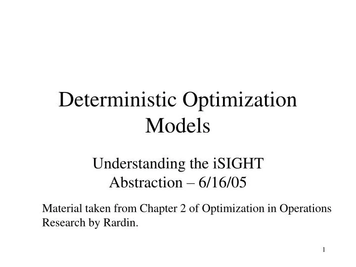
Deterministic Optimization Models. Understanding the iSIGHT Abstraction – 6/16/05. Material taken from Chapter 2 of Optimization in Operations Research by Rardin. Topics. Nomenclature Sample Problem Formulation and Intuitive Feel. Standard Problem Formulation

E N D
Deterministic Optimization Models Understanding the iSIGHT Abstraction – 6/16/05 Material taken from Chapter 2 of Optimization in OperationsResearch by Rardin.
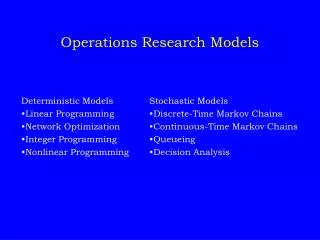
Topics • Nomenclature • Sample Problem Formulation and Intuitive Feel. • Standard Problem Formulation • Linear versus Nonlinear Optimization • Continuous vs. Discrete Optimization • Multiobjective Optimization
SimulationProgram Input Output Nomenclature Simulations C, Fortran, Java, Lisp Some take hours or days INPUTS Design Variables Independent Variables Starting Point lower bound upper bound Parameters Fixed values OUTPUTS Dependent Parameters Objective max or min Output Main Constraints >= or <= Output == Output
Two Crude Petroleum Example Two Crude Petroleum runs a small refinery on the Texas coast. The refinery distills crude petroleum from two sources, Saudi Arabia and Venezuela, into the three main products: gasoline, jet fuel and lubricants. The two crudes differ in chemical composition and yield different product mixes. Each barrel of Saudi crude yields 0.3 barrel of gasoline, 0.4 barrel of jet fuel, and 0.2 barrel of lubricants. Each barrel of Venezuelan crude yields 0.4 barrel of gasoline, 0.2 barrel of jet fuel and 0.3 barrel of lubricants. The remaining 10% is lost to refining. The crudes differ in cost and availability. Two Crude can purchase up to 9000 barrels per day from Saudia Arabia at $20 per barrel. Up to 6000 barrels per day of Venezuelan petroleum are available at the lower cost of $15 per barrel. Two Crude’s contracts require it to produce 2000 barrels per day of gasoline,1500 barrels per day of jet fuel and 500 barrels per day of lubricants.Develop an optimization model to satisfy these requirements at minimum cost. We will use this model throughout this lecture.
Two Crude Problem Description Petroleum refinery distills crude from Saudi and Venezuela Customer Demand(barrels) 2000 gas, 1500 jet, 500 lub Saudi Number of Barrels Purchased: ???? Cost Per Barrel: $20 Max Production Available: 9000 Refined barrel = .3 gas, .4 jet, .2 lub. Venezuela Number of Barrels Purchased: ???? Cost Per Barrel: $16 Max Production Available: 6000 Refined barrel = .4 gas, .2 jet, .3 lub. How can Two Crude Most Efficiently Meet Demands?
SimulationProgram Input Output Visual Tie In INPUTS Design Variables x1, x2 0 <=x1<=9 0 <=x2<=6 Parameters cost S 20, V 16 refined S .3, .4, .2 V .4, .2, .3 customer demand G 2, JF 1.5, L .5 OUTPUTS Cost Barrels Gas Barrels Jet Fuel Barrels Lubricants Objective min Cost Main Constraints Barrels Gas >= 2 Barrels JetFuel >= 1.5 Barrels Lub. >= .5 C ODE
General Mathematical Format The general form of a mathematical program or (single objective) optimization model is min or max f(x1,…,xn) Subject to: <= = >= g(x1,…,xn) bi i = 1,…,m Where f, g1,…,gm are given functions of decision variables x1,…,xn, and b1,…,bm are specified constant parameters.
Two Crude Petroleum Model min 20*x1 + 16*x2 s.t. 0.3*x1 + 0.4*x2 >= 2 0.4*x1 + 0.2*x2 >= 1.5 0.2*x1 + 0.3*x2 >= .500 x1 <= 9 x2 <= 6 x1,x2 >= 0 Design Variables? Variable Type Constraints? Main Constraints? Objective?
Class Exercise (2-1 Rardin) • Formulate the standard formulation • Show 2D Feasible Region and Objective Func. Contours The Joel Table Company sells two models of five leg tables. The basic version uses a wood top, requires 0.6 hours to assemble, and sells for a profit of $200. The deluxe version takes 1.5 hours to assemble because of glass top, and sells for a profit of $350. The company has 300 legs, 50 wood tops, 35 glass tops and 63 hours of assembly time. Joel wants to maximize profit and he knows that he can sell all you can make.
Linear Functions A function is linear if it is a constant weighted sum of decision variables. Otherwise it is nonlinear. f(x1,x2) = 20x1 + 15x2 f(w1,w2,w3) = w12 + 8w2 + w32
Recognizing Linear Functions Assuming x’s are decision variables, determine whethereach of the following functions are linear or nonlinear.
Linear Programs Defined An optimization model in functional form is a linearprogram (LP) if the (single) objective function f and all the constraint functions g1, … , gm are linear in the decision variables. Also, decision variables should be able to take on whole-number or fractional values.
Nonlinear Programs Defined An optimization model in functional form is a nonlinear program (NLP) if the (single) objective function f or any of the constraint functions g1,…,gm is nonlinear in the decision variables. Also, decision variables should be able to take on whole-number or fractional values.
Recognizing Linear and Nonlinear Programs Assuming y’s are decision variables and all other symbols are constant, determine if followingare linear programs or nonlinear programs.
Class Exercise (Rardin 2-18) Assuming that wj are decision variables and all other symbols Are constant, determine if each of the following is a linear programor a non linear program.
Discrete or Integer Programs Aka integer (linear or nonlinear) programs mixed integer (linear or nonlinear) programs combinatorial optimization problems A variable is discrete if it is limited to a fixed or countable set of values. Often the choices are only 0 or 1 (binary variable). A variable is continuous if it can take on any value in a specifiedinterval. When there is an option, such as when optimal variable magnitudes are likely to be large enough that fractions haveno practical importance, modeling with continuous variablesis prefered. (Does your program support option?)
Choosing Discrete Versus Continuous Variables Decide whether a discrete or continuous variable would bebest employed to model each of the following quantities. The operating temperature of a chemical process. The warehouse slot assigned a particular product The amount of money converted from yen to dollars The number of corvettes produced annually.
Constraints with Discrete Variables In choosing among a collection of 16 investment projects,variables 1 if project is selected wj = 0 otherwise Express each of the following constraints in terms of thesevariables. At least one of the first eight projects must be selected. At most three of the last eight projects must be selected. Either project 4 or project 9 must be selected, but not both Project 11 can be selected only if project 2 is also
Integer and Mixed Integer Programs An optimization model is an integer program (IP) if any ofits decision variables is discrete. If all variables are discrete,the model is a pure integer program; otherwise, it is a mixedinteger program. Case 1: wj >= 0, j=1,…,q Case 2: wj= 0 or 1, j=1,…,pwp+1>= 0 and integerCase 3: wj >= 0 j=1,…,pwp+1>= 0 and integer
Integer Linear and Integer Nonlinear Programs A discrete or integer programming model is an integer linearprogram (ILP) if its (single) objective function and all mainconstraints are linear.A discrete or integer programming model is an integer nonlinearprogram (INLP) if its (single) objective function or any of itsmain constraints is nonlinear.
Recognizing ILPs and INLPs Determine if each of the following is a LP, NLP, ILP, MINLP Max 3w1 + 14w2 – w3 s.t. w1 <= w2 w1 + w2 + w3 = 10 wj = 0 or 1 j=1,…,3 Min 3w1 + 9w2/ w3 s.t. w1 - w2<= 0 w1 + w2 + w3 = 10 w1 >= 0 w2 w3 >= 1 Min 3w1 + 14w2 – w3 s.t. w1w2<=1 w1 + w2 + w3 = 10 wj >= 0 j=1,…,3 w1 integer
Multiple Objectives All models considered so far have a single objective. A multiobjective optimization model maximizes or minimizesmore than one objective function at the same time. Multiple objectives for a automobile may be all of the following:max reliability f1(x1,…,xn) max mileage f2(x1,…,xn) min cost to produce f3(x1,…,xn)
NEOS Optimization Treehttp://www-fp.mcs.anl.gov/otc/Guide/OptWeb/
Lab Objectives • Define a iSIGHT calculation with inputs and outputs • Define a standard iSIGHT optimization problem formulation • Execute an optimization using default optimization plan
Lab Exercise GM Communications is choosing a cable for a new 16,000 meter telephone line. The following table shows the diameters available, along with the associated cost, resistance, and attenuation of each per meter. • Diameter Cost Resistance Attenuation • 4 0.092 0.279 0.00175 • 5 0.112 0.160 0.00130 • 6 0.141 0.120 0.00161 • 9 0.420 0.065 0.00095 • 12 0.719 0.039 0.00048 • The company wishes to choose the least cost combination of wires that will provide a new line with at most1600 ohms resistance and 8.5 decibels attenuation. • Formulate a mathematical programming model with three main constraints to choose an optimal combination of wires using decision variables x4, x5, x6, x9 and x12 • Put your formulation into iSIGHT. Create a task called Communication and create a Calculation to implement your equations. Formulate the iSIGHT Optimization Model in the Parameters window. If you have time then execute the model with the default task plan and write down the answer.
Lab Exercise The National Science Foundation (NSF) has received 4 proposals from professors to undertake new research in OR methods. Each proposal can be accepted for funding next year at the level (in thousands of dollars) shown in the following table or rejected. A total of $1 million is available for the year. Proposal 1 2 3 4 Funding 700 400 300 600 Score 85 70 62 93 Scores represent the estimated value of doing each body of research that was assigned by NSF’sadvisory panel. Formulate a discrete optimization model to decide what projects to accept to maximize total score within the available budget using decision variables pj = 1 if proposal j is selected and = 0 otherwise. Enter and set up the model in iSIGHT.
Lab 1 Follow up Optional slides
What does the iSIGHT client model support? Which of the following are supported by iSIGHT? Continuous Nonlinear Program Continuous Linear Program Integer Linear Program Integer Nonlinear Program Mixed Integer Linear Program Mixed Integer Nonlinear Program Multiple Objective Continuous Nonlinear Program Multiple Objective Mixed Integer Nonlinear Program
iSIGHT Abstraction • Single objective (combines multiple objectives into a single weighted objective called Objective) • Objective is considered a nonlinear function • Every constraint is considered nonlinear function • One constraint is always added by iSIGHT. TaskProcessStatus. You cannot remove it. • Design variables can be integer, discrete or continuous.
Supposed Difficulties of Classical Numerical Optimization • Computational time increases as the number of design variables increases. In addition, these methods tend to become numerically ill-conditioned. • Optimization techniques have no stored experience or intuition on which to draw. • Most algorithms will get stuck at a suboptimal design. • If the analysis program is not theoretically precise, the results may be misleading. Optimization will take advantage of analysis errors to provide mathematical design improvements. • Most optimization algorithms have difficulty dealing with discontinuous functions. • Convergence to optimal solution depends on chosen initial solution. • Algorithm efficient in solving one problem may not be efficient in solving a different optimization problem. • Many analysis/simulation programs were not written with automated design in mind.