1 / 0

Electromagnetic Models In Active And Passive Microwave Remote Sensing of Terrestrial Snow

Electromagnetic Models In Active And Passive Microwave Remote Sensing of Terrestrial Snow. Leung Tsang 1 , Xiaolan Xu 2 and Simon Yueh 2 1 Department of Electrical Engineering, University of Washington, Seattle, WA 2 Jet Propulsion Laboratory, Pasadena, CA. Radiative Transfer Equation.

rigg
Télécharger la présentation

Electromagnetic Models In Active And Passive Microwave Remote Sensing of Terrestrial Snow

An Image/Link below is provided (as is) to download presentation Download Policy: Content on the Website is provided to you AS IS for your information and personal use and may not be sold / licensed / shared on other websites without getting consent from its author. Content is provided to you AS IS for your information and personal use only. Download presentation by click this link. While downloading, if for some reason you are not able to download a presentation, the publisher may have deleted the file from their server. During download, if you can't get a presentation, the file might be deleted by the publisher.

E N D

Presentation Transcript


  1. Electromagnetic Models In Active And Passive Microwave Remote Sensing of Terrestrial Snow

    Leung Tsang1, Xiaolan Xu2 and Simon Yueh2 1Department of Electrical Engineering, University of Washington, Seattle, WA 2Jet Propulsion Laboratory, Pasadena, CA
  2. Radiative Transfer Equation
  3. Dense Media Radiative Transfer Equation (DMRT) Model 1) QCA Analytical Approximate Solution of Maxwell Equations Model 2) Foldy Lax equations Numerical Maxwell Equation Model (NMM3D) Since 2009, Model 3) Bicontinuous medium: Numerical Maxwell Equation Model (NMM3D) Bicontinuous media; Realistic microstructure of snow Comparisons With SnowSCAT
  4. DMRT Models
  5. Quasi-Crystalline Approximation (QCA) Lorentz-Lorenz law; Generalized Ewald-Oseen theorem Phase matrix, pair distribution function and structure factor Structure factor is the Fourier transform of
  6. Scattering Rate: QCA Compared With Classical Mie Scattering Diameter = 1.4 mm; Stickiness parameter τ=0.1; stickiness, adhere to form aggregates QCA sticky has weaker frequency dependence than Mie scattering
  7. Scattering Properties 1-2 polarization frame Phase matrix Scattering coefficient Mean cosine of scattering: angular distribution
  8. Phase Matrix: Angular DependenceQCA More Forward Scattering Frequency = 17.5 GHz; Diameter = 1.4 mm; Stickiness parameter τ=0.1 QCA predicts more forward scattering than Mie
  9. Scattering Properties Comparison
  10. Dense Media Radiative Transfer Equation (DMRT) Model 1) QCA Analytical Approximate Solution of Maxwell Equations Model 2) Foldy Lax equations Numerical Maxwell Equation Model (NMM3D) Model 3) Bicontinuous medium: Numerical Maxwell Equation Model (NMM3D) Bicontinuous media; Realistic microstructure of snow Comparisons With SnowSCAT
  11. Computer Generation Of Dense Sticky Particles Simulated sticky particles fv = 40% Random Shuffling Use Bonding States (a) Unbonded (b) Single-bond (c) Double-bond (d) Triple bond Kranendonk-Frenkel algorithm to calculate the probability , dependent on stickiness Aggregates formed from sequence of bonding
  12. Solutions of Maxwell Equations using Foldy-Lax equations field on particle i Mie scattering coefficients incident field field on particle j Green’s function
  13. Comparison Between Classical RT, DMRT / QCA and NMM3D NMM3D and QCA in agreement Weaker frequency dependence than independent scattering
  14. Model Comparison
  15. Dense Media Radiative Transfer Equation (DMRT) Model 1) QCA Analytical Approximate Solution of Maxwell Equations Model 2) Foldy Lax equations Numerical Maxwell Equation Model (NMM3D) Model 3) Bicontinuous medium: Numerical Maxwell Equation Model (NMM3D) Bicontinuous media; Realistic microstructure of snow Comparisons With SnowSCAT
  16. Bicontinuous Model: Computer Generation of Terrestrial Snow Generation: superimposing a large number of stochastic waves Cutting level α determined by fraction volume
  17. Bicontinuous Model: Generation Depth Hoar (30%): 3 cm * 3 cm picture A. Wiesmann, C. Mätzler, and T. Weise, "Radiometric and structural measurements of snow samples," Radio Sci., vol. 33, pp. 273-289, 1998. Computer generated snow pictures vs. real snow picture
  18. Numerical Solution Of Maxwell Equation Volume integral equation Discrete Dipole Approximation (DDA): in each cube Matrix equations Matrix-vector product by FFT
  19. Bicontinuous Parameters Bicontinuous parameters (α, <ζ>, b) One to one relation between α and fV Parameter <ζ> : inverse size Grain sizes decrease as <ζ> increases ζfollows Gamma distribution with mean value <ζ> Parameter b determines the size distribution Size distribution uniform for large b Broad size distributon for small b
  20. SSA and Correlation function of Bicontinuous Medium
  21. Real Snow Parameters Real snow parameters Fraction Volume (fV) or density (ρ): fV= ρsnow / ρice Auto Correlation Function (ACF) Specific Surface Area (SSA) Grain size Two grain size parameters D0: Equivalent grain size relating to SSA Dmax: Prevailing grain size, visually determined Empirical fit: Dmax=2.73D0
  22. Bicontinuous Model: Parameters Dependences on <ζ>
  23. Bicontinuous Model: Parameters Dependence on parameter b: b increases
  24. Bicontinuous Model: Correlation FunctionClose To Exponential Spatial auto correlation function
  25. Bicontinuous Model: Log Scale Correlation Function
  26. Bicontinuous Model: Specific Surface Area In Microwave Regime Example: <ζ>=6000 [m-1], b=1.5, fV=30% Bicontinuous SSA=71.8 [cm2/g] Analytical expression Numerical procedure: Use digitized picture, discretize according to microwave resolutions Count surface area
  27. Bicontinuous Model: Phase Matrix Mean cosine:
  28. Passive remote sensing: Effects Of ‘Mean Cosine’ Brightness temperature increases with for the same κS Physical temperature is 250 K Optical thickness = κSd; All curves have same κS
  29. Mean Cosine Comparisons Mean cosine > 0, means forward scattering is stronger than backward scattering
  30. Data Validation With SnowSCAT Data collected At IOA snow pit Radar backscattering and ground data: Dec. 28, 2010~Mar. 1, 2011 Data Time series backscattering Time series SWE SSA Density Depths of multilayer structure Grain sizes
  31. Comparisons With SnowSCAT Time series data for 9 different days in the same IOA snow pit Ground truth of data point #8 Bottom layer is the thickest layer Bottom layer has the largest grain size Typical values of measured SSA SSA measured in a different year from snow depth, density and grain size Bottom layers : 59 ~ 124 [cm2/g] Top and intermediate layers : 100 ~ 790 [cm2/g]
  32. Data Validation With SnowSCAT Bicontinuous input parameters
  33. Data Validation With SnowSCAT Bicontinuous extracted parameters
  34. Data Validation With SnowSCAT Co-polarization at 16.7 GHz
  35. DMRT Models Comparison
  36. Summary Bicontinuous model Computer Generation of snow microstructures Three parameters α, <ζ>, b Correlation function close to exponential correlation function and SSA Grain size indirectly, empirically related to correlation function and SSA Computer Generate structures and solve Maxwell equations numerically using DDA Compare with SnowSCATscatterometer data Using ground truth snow measurements
More Related