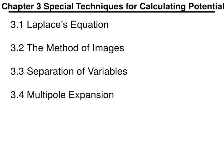
Chapter 3 Special Techniques for Calculating Potential

Chapter 3 Special Techniques for Calculating Potential 3.1 Laplace’s Equation 3.2 The Method of Images 3.3 Separation of Variables 3.4 Multipole Expansion

3.1 Laplace’s Equation 3.1.1 Introduction 3.1.2 Laplace’s Equation in One Dimension 3.1.3 Laplace’s Equation in Two Dimensions 3.1.4 Laplace’s Equation in Three Dimensions 3.1.5 Boundary Conditions and Uniqueness Theorems 3.1.6 Conducts and the Second Uniqueness Theorem

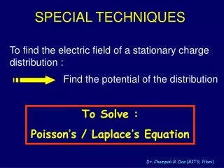
3.1.1 Introduction The primary task of electrostatics is to study the interaction (force) of a given stationary charges. since this integrals can be difficult (unless there is symmetry) we usually calculate This integral is often too tough to handle analytically.

3.1.1 In differential form Eq.(2.21): Poisson’s eq. • to solve a differential eq. we need boundary conditions. • In case of ρ = 0, Poisson’s eq. reduces to Laplace’s eq or The solutions of Laplace’s eq are called harmonic function.

3.1.2 Laplace’s Equation in One Dimension m, bare to be determined by B.C.s e.q., V=4 V=0 x 1 5 1. V(x)is the average of V(x + R)and V(x - R), for any R: 2. Laplace’s equation tolerates no local maxima or minima.

3.1.2 (2) Method of relaxation: • A numerical method to solve Laplace equation. • Starting V at the boundary and guess V on a grid of interior points. • Reassign each point with the average of its nearest neighbors. • Repeat this process till they converge.

3.1.2 (3) The example of relaxation

3.1.3 Laplace’s Equation in Two Dimensions A partial differential eq. : There is no general solution. The solution will be given in 3.3. We discuss certain general properties for now. The value of V at a point (x, y)is the average of those around the point. 2. V has no local maxima or minima; all extreme occur at the boundaries. 3. The method of relaxation can be applied.

3.1.4 Laplace’s Equation in Three Dimensions 1. The value of V at point P is the average value of V over a spherical surface of radius R centered at P: The same for a collection of q by the superposition principle. 2. As a consequence, V can have no local maxima or minima; the extreme values of V must occur at the boundaries. 3. The method of relaxation can be applied.

3.1.5 Boundary Conditions and Uniqueness Theorems in 1D, one end the other end Vb Va V is uniquely determined by its value at the boundary. First uniqueness theorem : the solution to Laplace’s equation in some region is uniquely determined, if the value of V is specified on all their surfaces; the outer boundary could be at infinity, where V is ordinarily taken to be zero.

3.1.5 Proof: Suppose V1, V2are solutions at boundary. at boundary V3 = 0 everywhere hence V1 = V2everywhere

3.1.5 The first uniqueness theorem applies to regions with charge. Proof. at boundary. Corollary : The potential in some region is uniquely determined if (a) the charge density throughout the region, and (b) the value of V on all boundaries, are specified.

3.1.6 Conductors and the Second Uniqueness Theorem • Second uniqueness theorem: In a region containing conductors and filled with a specified charge density ρ, the electric field is uniquely determined if the total charge on each conductor is given. (The region as a whole can be bounded by another conductor, or else unbounded.) Proof: Suppose both and are satisfied. and

3.1.6 define for V3 is a constant over each conducting surface

3.2 The Method of Images 3.2.1 The Classical Image Problem 3.2.2 The Induced Surface Charge 3.2.3 Force and Energy 3.2.4 Other Image Problems

3.2.1 The Classical Image Problem B.C. What is V (z>0) ? The first uniqueness theorem guarantees that there is only one solution. If we can get one any means, that is the only answer.

3.2.1 Trick : Only care z > 0 z < 0 is not of concern V(z=0) = const = 0 in original problem for

3.2.2 The Induced Surface Charge Eq.(2.49)

3.2.2 total induced surface charge Q=-q

3.2.3 Force and Energy The charge q is attracted toward the plane. The force of attraction is With 2 point charges and no conducting plane, the energy is Eq.(2.36)

3.2.3 (2) For point charge q and the conducting plane at z = 0 the energy is half of the energy given at above, because the field exist only at z≥ 0 ,and is zero at z < 0 ; that is or

3.2.4 Other Image Problems Stationary distribution of charge

3.2.4 (2) Conducting sphere of radius R Image charge at

3.2.4 (3) Force [Note : how about conducting circular cylinder?]

3.3 Separation of Variables 3.3.0Fourier series and Fourier transform 3.3.1 Cartesian Coordinate 3.3.2 Spherical Coordinate

3.3.0Fourier series and Fourier transform Basic set of unit vectors in a certain coordinate can express any vector uniquely in the space represented by the coordinate. e.g. in 3D. Cartesian Coordinate. are unique because are orthogonal. 0 = 1 Completeness: a set of function is complete. if for any function Orthogonal: a set of functions is orthogonal for if for =const

3.3.0 (2) A complete and orthogonal set of functions forms a basic set of functions. e.g. odd even sin(nx) is a basic set of functions for any odd function. cos(nx) is a basic set of functions for any even function. sin(nx) and cos(nx) are a basic set of functions for any functions.

3.3.0 (3) , ; for any odd even odd even [sinkx] [coskx] Fourier transform and Fourier series

3.3.0 (4) Proof

3.3.0 (5) B0 2p for k = 0 Bk p for k = 1, 2, …

3.3.1 Cartesian Coordinate Use the method of separation of variables to solve the Laplace’s eq. Example 3 Find the potential inside this “slot”? Laplace’s eq. set

set 3.3.1 (2) f and g are constant so

3.3.1 (3) B.C. (iv) B.C. (i) B.C. (ii) The principle of superposition B.C. (iii) A fourier series for odd function

For 3.3.1 (4)

3.4 Multipole Expansion 3.4.1 Approximate Potentials at Large distances 3.4.2 The Monopole and Dipole Terms 3.4.3 Origin of Coordinates in Multipole Expansions 3.4.4 The Electric Field of a Dipole

3.4.1 Approximate Potentials at Large distances Example 3.10 A dipole (Fig 3.27). Find the approximate potential at points far from the dipole.

3.4.1 Example 3.10 For an arbitrary localized charge distribution. Find a systematic expansion of the potential?

3.4.1(2) Monopole term Dipole term Quadrupole term Multipole expansion

3.4.2 The Monopole and Dipole Terms monopole dominates if r >> 1 dipole dipole moment (vector) A physical dipole is consist of a pair of equal and opposite charge,

3.4.3 Origin of Coordinates in Multipole Expansions if

3.4.4 The Electric Field of a Dipole A pure dipole

Chapter 3 Special Techniques for Calculating Potential