Download
1 / 214
2.14k likes | 2.29k Vues
Development and testing of a global forecast model … configured on a horizontally icosahedral, vertically quasi-material (“flow-following”) grid. Today’s presenters: Jin Lee and Rainer Bleck NOAA Earth System Research Lab, Boulder, Colorado. NOAA/ESRL F low-following- finite-volume

E N D
Development and testing of a global forecast model… configured on a horizontally icosahedral, vertically quasi-material (“flow-following”) grid Today’s presenters: Jin Lee and Rainer Bleck NOAA Earth System Research Lab, Boulder, Colorado
NOAA/ESRL Flow-following- finite-volume Icosahedral Model FIM Sandy MacDonald Rainer Bleck Stan Benjamin Jian-Wen Bao John M. Brown Jacques Middlecoff Jin-luen Lee Earth System Research Laboratory
Topics covered: • Introduction (Rainer) • Horizontal discretization: the icosahedral grid; 2-D results (Jin) • Vertical discretization: the hybrid-isentropic grid (Rainer) • 3-D Results, conclusions, and outlook (Jin)
Topics covered: • Introduction (Rainer) • Horizontal discretization: the icosahedral grid; 2-D results (Jin) • Vertical discretization: the hybrid-isentropic grid (Rainer) • 3-D Results, conclusions, and outlook (Jin)
ESRL Flow-following, finite volume Icosahedral Model (FIM) Icosahedral grid, with spring dynamics implementation Finite volume, flux form equations in horizontal (planned - Piecewise Parabolic Method) Hybrid isentropic-sigma ALE vertical coordinate (arbitrary Lagrangian-Eulerian) Nonhydrostatic (not initially) Earth System Modeling Framework
Why Icosahedral Finite-Volume (FV) model ? 1) Icosahedral + FV approach provides conservation. 2) Icos quasi-uniform grid is free of pole problems. 3) Legendre polynomials become inefficient at high resol. 4) Spectral models require global communication which is inefficient on MPP with distributed memory. 5) Spectral models tend to generate noisy tracer transport. Since Icosahedral models are based on a local numerical scheme, they are free of above problems 3 – 5.
Icosahedral Grid Generation N=((2**n)**2)*10 + 2 ; 5th level – n=5 N=10242 ~ 240km; max(d)/min(d)~1.2 6th level – n=6 N=N=40962 ~ 120km; 7th level – n=7N=163842 ~60km 8th level – n=8N=655,362 ~30km; 9th level – n=9N=2,621,442 ~15km
N=(m**2)*10 + 2 “m” is any integer ratio between arc(AB~8000 km) and target resolution. e.g., for dx~20 km, then m=8000/20=400 N=(400**2)*10+2~1.6 million points. high granularity possible with icosa-hedral model Sadourny, Arakawa, Mintz, MWR (1968)
Numerics of the Icosahedral SWE • Finite-Volume operators including (i) Vorticity operator based on Stoke theorem, (ii) Divergence operator based on Gauss theorem, (iii) Gradient operator based on Green’s theorem. • Explicit 3rd-order Adams-Bashforth time differencing. • Icosahedral grid is optimized with springdynamics.
Finite volume flux computation: - flux into each cell from surrounding donor cells
I) Shallow-water dynamics are evaluated with the standard tests of Williamson et. al. (1992) including: .Advection of cosine bell over poles.Steady state nonlinear geostrophic flow.Forced nonlinear translating.Zonal flow over an isolated mountain.Rossby-Haurwitz solution II) Monotonicity and positive-definiteness achieved by.Zalesak (1979) flux corrected transport (FCT).Demonstrated with emerging seamount experiment III) Tracer eqns are solved by same FCTroutine.tracer transport is tested with pot.vort. advection
The following 2 tests are run with level 5 grid on 10242 grid points, i.e., dx~240 km. .Rossby-Haurwitz wave .Emerging seamount
Mass conservation in Rossby-Haurwitz solution Time integration
Emerging seamount experiment to test FCT in the limit of zero layer thickness
Shallow water equations, uniform density, water depth 3000m. Initial conditions: state of rest. Seamount at 30 S growing to 3500 m in 24 hrs. Zero thickness (dry land) after day 3 90N Eq 90S
Shallow water equations, uniform density, water depth 3000m. Initial conditions: state of rest. Seamount at 30 S growing to 3500 m in 24 hrs. Zero thickness (dry land) after day 3
Shallow water equations, uniform density, water depth 3000m. Initial conditions: state of rest. Seamount at 30 S growing to 3500 m in 24 hrs. Zero thickness (dry land) after day 3
Shallow water equations, uniform density, water depth 3000m. Initial conditions: state of rest. Seamount at 30 S growing to 3500 m in 24 hrs. Zero thickness (dry land) after day 3
Shallow water equations, uniform density, water depth 3000m. Initial conditions: state of rest. Seamount at 30 S growing to 3500 m in 24 hrs. Zero thickness (dry land) after day 3
Topics covered: • Introduction (Rainer) • Horizontal discretization: the icosahedral grid; 2-D results (Jin) • Vertical discretization: the hybrid-isentropic grid (Rainer) • 3-D Results, conclusions, and outlook (Jin)
Major Pros: No uncontrolled diabatic mixing (in the vertical and horizontal) Numerical dispersion errors associated with vertical transport are minimized Optimal finite-difference representation of frontal zones & frontogenesis Major Cons: Coordinate-ground intersections are inevitable (atmosphere doesn’t fit snugly into x,y,q grid box) Poor vertical resolution in weakly stratified regions Elaborate transport operators needed to achieve conservation Lagrangian vertical coordinate:Pros and Cons(“Lagrangian” = isentropic in atmospheric applications)
The x,y,q grid box north east q .
Major Cons: Coordinate-ground intersections are inevitable (atmosphere doesn’t fit snugly into x,y,q grid box) Poor vertical resolution in weakly stratified regions Fixes: • Reassign grid points from underground portion of x,y,q grid box to above-ground “s” surfaces • Low stratification => large portion of x,y,q grid box is underground => no shortage of grid points available for re-deployment as s points => A “hybrid” grid appears to have distinct advantages – bothfrom a grid-economy and a vertical resolution perspective
"Hybrid" means different things to different people: - linear combination of 2 or more conventional coordinates (examples: p+sigma, p+theta+sigma) - ALE (Arbitrary Lagrangian-Eulerian) coordinate ALE maximizes size of isentropic subdomain.
ALE: “Arbitrary Lagrangian-Eulerian” coordinate • Original concept (Hirt et al., 1974): maintain Lagrangian character of coordinate but “re-grid” intermittently to keep grid points from fusing. • In RUC, FIM, and HYCOM, we apply ALE in the vertical only and re-grid for 2 reasons: • (1) to maintain minimum layer thickness; • (2) to nudge an entropy-related thermodynamic variable toward a prescribed layer-specific “target” value by importing mass from above or below. • Process (2) renders the grid quasi-isentropic
Main design element of layer models: Height (alias layer thickness) is treated as dependent variable. • needed: a new independent variable capable of representing 3rd (vertical) model dimension. Call this variable “s”. Having increased the number of unknowns by 1 (layer thickness), we need 1 additional equation. The logical choice is an equation linking “s” to other variables. • popular example: s = potential temperature Hence ….