Download
1 / 62
620 likes | 701 Vues
Chapter 4 Network Layer. 4. 1 Introduction 4.2 Virtual circuit and datagram networks 4.3 What’s inside a router 4.4 IP: Internet Protocol Datagram format IPv4 addressing ICMP IPv6. 4.5 Routing algorithms Link state Distance Vector Hierarchical routing 4.6 Routing in the Internet RIP

E N D
Chapter 4Network Layer Network Layer
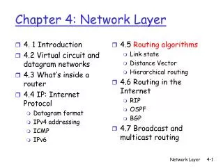
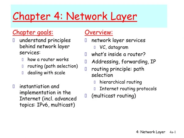
4. 1 Introduction 4.2 Virtual circuit and datagram networks 4.3 What’s inside a router 4.4 IP: Internet Protocol Datagram format IPv4 addressing ICMP IPv6 4.5 Routing algorithms Link state Distance Vector Hierarchical routing 4.6 Routing in the Internet RIP OSPF BGP 4.7 Broadcast and multicast routing Chapter 4: Network Layer Network Layer
NAT: Network Address Translation rest of Internet local network (e.g., home network) 10.0.0/24 10.0.0.1 10.0.0.4 10.0.0.2 138.76.29.7 10.0.0.3 Datagrams with source or destination in this network have 10.0.0/24 address for source, destination (as usual) All datagrams leaving local network have same single source NAT IP address: 138.76.29.7, different source port numbers Network Layer
NAT: Network Address Translation • Motivation: local network uses just one IP address as far as outside world is concerned: • range of addresses not needed from ISP: just one IP address for all devices • can change addresses of devices in local network without notifying outside world • can change ISP without changing addresses of devices in local network • devices inside local net not explicitly addressable, visible by outside world (a security plus). Network Layer
NAT: Network Address Translation Implementation: NAT router must: • outgoing datagrams:replace (source IP address, port #) of every outgoing datagram to (NAT IP address, new port #) remote clients/servers will respond using (NAT IP address, new port #) as destination addr. • remember (in NAT translation table) every (source IP address, port #) to (NAT IP address, new port #) translation pair • incoming datagrams:replace (NAT IP address, new port #) in dest fields of every incoming datagram with corresponding (source IP address, port #) stored in NAT table Network Layer
1 S: 10.0.0.1, 3345 D: 128.119.40.186, 80 1:host 10.0.0.1 sends datagram to 128.119.40.186, 80 NAT: Network Address Translation 10.0.0.1 10.0.0.4 10.0.0.2 138.76.29.7 10.0.0.3 Network Layer
1 2 S: 10.0.0.1, 3345 D: 128.119.40.186, 80 S: 138.76.29.7, 5001 D: 128.119.40.186, 80 1:host 10.0.0.1 sends datagram to 128.119.40.186, 80 2:NAT router changes datagram source addr from 10.0.0.1, 3345 to 138.76.29.7, 5001, updates table NAT: Network Address Translation NAT translation table WAN side addr LAN side addr 138.76.29.7, 5001 10.0.0.1, 3345 …… …… 10.0.0.1 10.0.0.4 10.0.0.2 138.76.29.7 10.0.0.3 Network Layer
1 3 2 S: 10.0.0.1, 3345 D: 128.119.40.186, 80 S: 138.76.29.7, 5001 D: 128.119.40.186, 80 1:host 10.0.0.1 sends datagram to 128.119.40.186, 80 2: NAT router changes datagram source addr from 10.0.0.1, 3345 to 138.76.29.7, 5001, updates table S: 128.119.40.186, 80 D: 138.76.29.7, 5001 NAT: Network Address Translation NAT translation table WAN side addr LAN side addr 138.76.29.7, 5001 10.0.0.1, 3345 …… …… 10.0.0.1 10.0.0.4 10.0.0.2 138.76.29.7 10.0.0.3 3:Reply arrives dest. address: 138.76.29.7, 5001 Network Layer
2 4 1 3 S: 138.76.29.7, 5001 D: 128.119.40.186, 80 S: 10.0.0.1, 3345 D: 128.119.40.186, 80 1:host 10.0.0.1 sends datagram to 128.119.40.186, 80 2:NAT router changes datagram source addr from 10.0.0.1, 3345 to 138.76.29.7, 5001, updates table S: 128.119.40.186, 80 D: 10.0.0.1, 3345 S: 128.119.40.186, 80 D: 138.76.29.7, 5001 NAT: Network Address Translation NAT translation table WAN side addr LAN side addr 138.76.29.7, 5001 10.0.0.1, 3345 …… …… 10.0.0.1 10.0.0.4 10.0.0.2 138.76.29.7 10.0.0.3 4:NAT router changes datagram dest addr from 138.76.29.7, 5001 to 10.0.0.1, 3345 3:Reply arrives dest. address: 138.76.29.7, 5001 Network Layer
NAT: Network Address Translation • 16-bit port-number field: • 60,000 simultaneous connections with a single LAN-side address! • NAT is controversial: • routers should only process up to layer 3 • violates end-to-end argument • NAT possibility must be taken into account by app designers, e.g., P2P applications • address shortage should instead be solved by IPv6 Network Layer
NAT traversal problem • client wants to connect to server with address 10.0.0.1 • server address 10.0.0.1 local to LAN (client can’t use it as destination addr) • only one externally visible NATed address: 138.76.29.7 • solution 1: statically configure NAT to forward incoming connection requests at given port to server • e.g., (123.76.29.7, port 2500) always forwarded to 10.0.0.1 port 25000 10.0.0.1 Client ? 10.0.0.4 138.76.29.7 NAT router Network Layer
NAT traversal problem • solution 2: Universal Plug and Play (UPnP) Internet Gateway Device (IGD) Protocol. Allows NATed host to: • learn public IP address (138.76.29.7) • add/remove port mappings (with lease times) 10.0.0.1 IGD 10.0.0.4 138.76.29.7 NAT router Network Layer
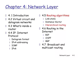
4. 1 Introduction 4.2 Virtual circuit and datagram networks 4.3 What’s inside a router 4.4 IP: Internet Protocol Datagram format IPv4 addressing ICMP IPv6 4.5 Routing algorithms Link state Distance Vector Hierarchical routing 4.6 Routing in the Internet RIP OSPF BGP 4.7 Broadcast and multicast routing Chapter 4: Network Layer Network Layer
used by hosts & routers to communicate network-level information error reporting: unreachable host, network, port, protocol echo request/reply (used by ping) network-layer “above” IP: ICMP msgs carried in IP datagrams ICMP message: type, code plus first 8 bytes of IP datagram causing error ICMP: Internet Control Message Protocol TypeCodedescription 0 0 echo reply (ping) 3 0 dest. network unreachable 3 1 dest host unreachable 3 2 dest protocol unreachable 3 3 dest port unreachable 3 6 dest network unknown 3 7 dest host unknown 4 0 source quench (congestion control - not used) 8 0 echo request (ping) 9 0 route advertisement 10 0 router discovery 11 0 TTL expired 12 0 bad IP header Network Layer
Source sends series of UDP segments to dest first has TTL =1 second has TTL=2, etc. unlikely port number When nth datagram arrives to nth router: router discards datagram and sends to source an ICMP message (type 11, code 0) ICMP message includes name of router & IP address when ICMP message arrives, source calculates RTT traceroute does this 3 times Stopping criterion UDP segment eventually arrives at destination host destination returns ICMP “port unreachable” packet (type 3, code 3) when source gets this ICMP, stops. Traceroute and ICMP Network Layer
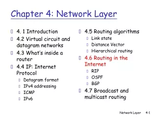
4. 1 Introduction 4.2 Virtual circuit and datagram networks 4.3 What’s inside a router 4.4 IP: Internet Protocol Datagram format IPv4 addressing ICMP IPv6 4.5 Routing algorithms Link state Distance Vector Hierarchical routing 4.6 Routing in the Internet RIP OSPF BGP 4.7 Broadcast and multicast routing Chapter 4: Network Layer Network Layer
IPv6 • Initial motivation:32-bit address space soon to be completely allocated. • Additional motivation: • header format helps speed processing/forwarding • header changes to facilitate QoS IPv6 datagram format: • fixed-length 40 byte header • no fragmentation allowed Network Layer
IPv6 Header (Cont) Priority: identify priority among datagrams in flow Flow Label: identify datagrams in same “flow.” (concept of“flow” not well defined). Next header: identify upper layer protocol for data pri ver flow label hop limit payload len next hdr source address (128 bits) destination address (128 bits) data 32 bits Network Layer
Other Changes from IPv4 • Checksum:removed entirely to reduce processing time at each hop • Options: allowed, but outside of header, indicated by “Next Header” field • ICMPv6: new version of ICMP • additional message types, e.g. “Packet Too Big” • multicast group management functions Network Layer
Transition From IPv4 To IPv6 • Not all routers can be upgraded simultaneous • no “flag days” • How will the network operate with mixed IPv4 and IPv6 routers? • Tunneling: IPv6 carried as payload in IPv4 datagram among IPv4 routers Network Layer
F A B E F E B A tunnel Logical view: IPv6 IPv6 IPv6 IPv6 Physical view: IPv6 IPv6 IPv6 IPv6 IPv4 IPv4 Tunneling Network Layer
Flow: X Src: A Dest: F data Flow: X Src: A Dest: F data Flow: X Src: A Dest: F data Flow: X Src: A Dest: F data A B E F F A B E C D Src:B Dest: E Src:B Dest: E Tunneling tunnel Logical view: IPv6 IPv6 IPv6 IPv6 Physical view: IPv6 IPv6 IPv6 IPv6 IPv4 IPv4 A-to-B: IPv6 E-to-F: IPv6 B-to-C: IPv6 inside IPv4 B-to-C: IPv6 inside IPv4 Network Layer
4. 1 Introduction 4.2 Virtual circuit and datagram networks 4.3 What’s inside a router 4.4 IP: Internet Protocol Datagram format IPv4 addressing ICMP IPv6 4.5 Routing algorithms Link state Distance Vector Hierarchical routing 4.6 Routing in the Internet RIP OSPF BGP 4.7 Broadcast and multicast routing Chapter 4: Network Layer Network Layer
routing algorithm local forwarding table header value output link 0100 0101 0111 1001 3 2 2 1 value in arriving packet’s header 1 0111 2 3 Interplay between routing, forwarding Network Layer
5 3 5 2 2 1 3 1 2 1 x z w y u v Graph abstraction Graph: G = (N,E) N = set of routers = { u, v, w, x, y, z } E = set of links ={ (u,v), (u,x), (v,x), (v,w), (x,w), (x,y), (w,y), (w,z), (y,z) } Remark: Graph abstraction is useful in other network contexts Example: P2P, where N is set of peers and E is set of TCP connections Network Layer
5 3 5 2 2 1 3 1 2 1 x z w y u v Graph abstraction: costs • c(x,x’) = cost of link (x,x’) • - e.g., c(w,z) = 5 • cost could always be 1, or • inversely related to bandwidth, • or inversely related to • congestion Cost of path (x1, x2, x3,…, xp) = c(x1,x2) + c(x2,x3) + … + c(xp-1,xp) Question: What’s the least-cost path between u and z ? Routing algorithm: algorithm that finds least-cost path Network Layer
Global or decentralized information? Global: all routers have complete topology, link cost info “link state” algorithms Decentralized: router knows physically-connected neighbors, link costs to neighbors iterative process of computation, exchange of info with neighbors “distance vector” algorithms Static or dynamic? Static: routes change slowly over time Dynamic: routes change more quickly periodic update in response to link cost changes Routing Algorithm classification Network Layer
4. 1 Introduction 4.2 Virtual circuit and datagram networks 4.3 What’s inside a router 4.4 IP: Internet Protocol Datagram format IPv4 addressing ICMP IPv6 4.5 Routing algorithms Link state Distance Vector Hierarchical routing 4.6 Routing in the Internet RIP OSPF BGP 4.7 Broadcast and multicast routing Chapter 4: Network Layer Network Layer
Dijkstra’s algorithm net topology, link costs known to all nodes accomplished via “link state broadcast” all nodes have same info computes least cost paths from one node (‘source”) to all other nodes gives forwarding table for that node iterative: after k iterations, know least cost path to k dest.’s Notation: c(x,y): link cost from node x to y; = ∞ if not direct neighbors D(v): current value of cost of path from source to dest. v p(v): predecessor node along path from source to v N': set of nodes whose least cost path definitively known A Link-State Routing Algorithm Network Layer
Dijsktra’s Algorithm 1 Initialization: 2 N' = {u} 3 for all nodes v 4 if v adjacent to u 5 then D(v) = c(u,v) 6 else D(v) = ∞ 7 8 Loop 9 find w not in N' such that D(w) is a minimum 10 add w to N' 11 update D(v) for all v adjacent to w and not in N' : 12 D(v) = min( D(v), D(w) + c(w,v) ) 13 /* new cost to v is either old cost to v or known 14 shortest path cost to w plus cost from w to v */ 15 until all nodes in N' Network Layer
Dijkstra’s algorithm: example 9 ∞ ∞ 3,u 5,u 7,u 7 5 4 8 3 w x z u y v 2 3 4 7 D(v) p(v) D(w) p(w) D(x) p(x) D(y) p(y) D(z) p(z) Step N' u 0 5 3 Step0 7 Network Layer
Dijkstra’s algorithm: example 9 11,w ∞ ∞ ∞ 3,u 5,u 5,u 6,w 7,u 7 5 4 8 3 w x z y u v 2 3 4 7 D(v) p(v) D(w) p(w) D(x) p(x) D(y) p(y) D(z) p(z) Step N' u 0 uw 1 5 7 Step1 11 3 6 7 Network Layer
Dijkstra’s algorithm: example 11,w 9 14,x 11,w ∞ ∞ ∞ 3,u 5,u 5,u 6,w 6,w 7,u 7 5 4 8 3 w x z u y v 2 3 4 7 D(v) p(v) D(w) p(w) D(x) p(x) D(y) p(y) D(z) p(z) Step N' u 0 uw 1 uwx 2 Step2 5 14 12 3 11 6 Network Layer
Dijkstra’s algorithm: example 11,w 9 14,x 11,w ∞ ∞ ∞ 3,u 5,u 5,u 6,w 6,w 7,u 7 5 4 8 3 w x z u y v 2 3 4 7 10,v 14,x D(v) p(v) D(w) p(w) D(x) p(x) D(y) p(y) D(z) p(z) Step N' u 0 uw 1 uwx 2 uwxv 3 5 14 11 3 10 6 Step3 Network Layer
Dijkstra’s algorithm: example 11,w 9 14,x 11,w ∞ ∞ ∞ 3,u 5,u 5,u 6,w 6,w 7,u 7 5 4 8 3 w x z u y v 2 3 4 7 10,v 14,x D(v) p(v) D(w) p(w) D(x) p(x) D(y) p(y) D(z) p(z) Step N' u 0 uw 1 uwx 2 uwxv 3 5 uwxvy 4 12,y 12 14 10 3 6 Network Layer
Dijkstra’s algorithm: example 11,w 9 14,x 11,w ∞ ∞ ∞ 3,u 5,u 5,u 6,w 6,w 7,u 7 5 4 8 3 w x z u y v 2 3 4 7 10,v 14,x D(v) p(v) D(w) p(w) D(x) p(x) D(y) p(y) D(z) p(z) Step N' u 0 uw 1 uwx 2 uwxv 3 uwxvy 4 12,y uwxvyz 5 Notes: • construct shortest path tree by tracing predecessor nodes • ties can exist (can be broken arbitrarily) Network Layer
x z w u y v Dijkstra’s algorithm: another example D(v),p(v) 2,u 2,u 2,u D(x),p(x) 1,u D(w),p(w) 5,u 4,x 3,y 3,y D(y),p(y) ∞ 2,x Step 0 1 2 3 4 5 N' u ux uxy uxyv uxyvw uxyvwz D(z),p(z) ∞ ∞ 4,y 4,y 4,y 5 3 5 2 2 1 3 1 2 1 Network Layer
x z w u y v destination link (u,v) v (u,x) x y (u,x) (u,x) w z (u,x) Dijkstra’s algorithm: example (2) Resulting shortest-path tree from u: Resulting forwarding table in u: Network Layer
Algorithm complexity: n nodes each iteration: need to check all nodes, w, not in N n(n+1)/2 comparisons: O(n2) more efficient implementations possible: O(nlogn) Oscillations possible: e.g., link cost = amount of carried traffic A A A A D D D D B B B B C C C C 1 1+e 2+e 0 2+e 0 2+e 0 0 0 1 1+e 0 0 1 1+e e 0 0 0 e 1 1+e 0 1 1 e … recompute … recompute routing … recompute initially Dijkstra’s algorithm, discussion Network Layer
4. 1 Introduction 4.2 Virtual circuit and datagram networks 4.3 What’s inside a router 4.4 IP: Internet Protocol Datagram format IPv4 addressing ICMP IPv6 4.5 Routing algorithms Link state Distance Vector Hierarchical routing 4.6 Routing in the Internet RIP OSPF BGP 4.7 Broadcast and multicast routing Chapter 4: Network Layer Network Layer
Distance Vector Algorithm • Based on Bellman-Ford equation • Define dx(y) := cost of least-cost path from x to y c(x,y) := cost of direct link from x to y • Then, dx(y) = min {c(x,v) + dv(y) } where min is taken over all neighbors v of x Network Layer
5 3 5 2 2 1 3 1 2 1 x z w u y v Bellman-Ford example Consider a path from u to z Clearly, dv(z) = 5, dx(z) = 3, dw(z) = 3 B-F equation says: du(z) = min { c(u,v) + dv(z), c(u,x) + dx(z), c(u,w) + dw(z) } = min {2 + 5, 1 + 3, 5 + 3} = 4 Network Layer
Distance Vector Algorithm • Dx(y) = estimate of least cost from x to y • x maintains distance vector Dx = [Dx(y): y є N ] • node x: • knows cost to each neighbor v: c(x,v) • maintains its neighbors’ distance vectors. For each neighbor v, x maintains Dv = [Dv(y): y є N ] Network Layer
Distance vector algorithm (4) Basic idea: • Every node v keeps vector (DV) of least costs to other nodes • These are estimates, Dx(y) • from time-to-time, each node sends its own distance vector estimate to neighbors • when x receives new DV estimate from neighbor, it updates its own DV using B-F equation: Dx(y) ← minv{c(x,v) + Dv(y)} for each node y ∊ N • under minor, natural conditions, the estimate Dx(y) converge to the actual least cost dx(y) Network Layer
Iterative, asynchronous: each local iteration caused by: local link cost change DV update message from neighbor Distributed: each node notifies neighbors only when its DV changes neighbors then notify their neighbors if necessary Distance Vector Algorithm (5) Each node: waitfor (change in local link cost or msg from neighbor) recompute estimates if DV to any dest has changed, notify neighbors Network Layer
cost to x y z x 0 2 7 y from ∞ ∞ ∞ z ∞ ∞ ∞ 2 1 7 z x y node x table node y table cost to x y z x ∞ ∞ ∞ 2 0 1 y from Step 1: Initialization Initialize costs of direct links Set to ∞ costs from neighbours z ∞ ∞ ∞ node z table cost to x y z x ∞ ∞ ∞ y from ∞ ∞ ∞ z 7 1 0 time Network Layer
cost to x y z x 0 2 7 y from ∞ ∞ ∞ z ∞ ∞ ∞ 2 1 7 z x y Dx(z) = min{c(x,y) + Dy(z), c(x,z) + Dz(z)} = min{2+1 , 7+0} = 3 Dx(y) = min{c(x,y) + Dy(y), c(x,z) + Dz(y)} = min{2+0 , 7+1} = 2 node x table cost to x y z x 0 2 3 y from 2 0 1 z 7 1 0 node y table cost to x y z Step 2: Exchange DV and iterate -In first iteration, node x saves neighbours’ DVs -Then, it checks path costs to all nodes using received DVs -E.g. new cost Dx(z) is obtained by adding costs marked red x ∞ ∞ ∞ 2 0 1 y from z ∞ ∞ ∞ node z table cost to x y z x ∞ ∞ ∞ y from ∞ ∞ ∞ z 7 1 0 time Network Layer
cost to x y z x 0 2 7 y from ∞ ∞ ∞ z ∞ ∞ ∞ 2 1 7 z x y node x table cost to cost to x y z x y z x 0 2 3 x 0 2 3 y from 2 0 1 y from 2 0 1 z 7 1 0 z 3 1 0 node y table cost to cost to cost to x y z x y z x y z x ∞ ∞ x 0 2 7 ∞ 2 0 1 x 0 2 3 y y from 2 0 1 y from from 2 0 1 z z ∞ ∞ ∞ 7 1 0 z 3 1 0 node z table cost to cost to cost to x y z x y z x y z x 0 2 7 x 0 2 3 x ∞ ∞ ∞ y y 2 0 1 from from y 2 0 1 from ∞ ∞ ∞ z z z 3 1 0 3 1 0 7 1 0 time Network Layer
1 4 1 50 x z y Distance Vector: link cost changes Link cost changes: • node detects local link cost change • updates routing info, recalculates distance vector • if DV changes, notify neighbors Network Layer
1 4 1 50 x z y Distance Vector: link cost changes Link cost changes: • node detects local link cost change • updates routing info, recalculates distance vector • if DV changes, notify neighbors t0 : y detects link-cost change, updates its DV, informs its neighbors. Network Layer