Download
1 / 21
230 likes | 1.71k Vues
Slides Prepared by JOHN S. LOUCKS ST. EDWARD’S UNIVERSITY. Chapter 3 Linear Programming: Sensitivity Analysis and Interpretation of Solution. Introduction to Sensitivity Analysis Graphical Sensitivity Analysis Sensitivity Analysis: Computer Solution Simultaneous Changes.

E N D
Slides Prepared by JOHN S. LOUCKS ST. EDWARD’S UNIVERSITY
Chapter 3 Linear Programming: Sensitivity Analysis and Interpretation of Solution • Introduction to Sensitivity Analysis • Graphical Sensitivity Analysis • Sensitivity Analysis: Computer Solution • Simultaneous Changes
Standard Computer Output Software packages such as The Management Scientist and Microsoft Excel provide the following LP information: • Information about the objective function: • its optimal value • coefficient ranges (ranges of optimality) • Information about the decision variables: • their optimal values • their reduced costs • Information about the constraints: • the amount of slack or surplus • the dual prices • right-hand side ranges (ranges of feasibility)
Standard Computer Output • In the previous chapter we discussed: • objective function value • values of the decision variables • reduced costs • slack/surplus • In this chapter we will discuss: • changes in the coefficients of the objective function • changes in the right-hand side value of a constraint
Sensitivity Analysis • Sensitivity analysis (or post-optimality analysis) is used to determine how the optimal solution is affected by changes, within specified ranges, in: • the objective function coefficients • the right-hand side (RHS) values • Sensitivity analysis is important to the manager who must operate in a dynamic environment with imprecise estimates of the coefficients. • Sensitivity analysis allows him to ask certain what-ifquestions about the problem.
Objective Function Coefficients • The range of optimality for each coefficient provides the range of values over which the current solution will remain optimal. • Managers should focus on those objective coefficients that have a narrow range of optimality and coefficients near the endpoints of the range.
Right-Hand Sides • The improvement in the value of the optimal solution per unit increase in the right-hand side is called the shadow price. • The range of feasibility is the range over which the shadow price is applicable. • As the RHS increases, other constraints will become binding and limit the change in the value of the objective function.
Example : Olympic Bike Co. Olympic Bike is introducing two new lightweight bicycle frames, the Deluxe and the Professional, to be made from special aluminum and steel alloys. The anticipated unit profits are $10 for the Deluxe and $15 for the Professional. The number of pounds of each alloy needed per frame is summarized on the next slide.
Example 2: Olympic Bike Co. A supplier delivers 100 pounds of the aluminum alloy and 80 pounds of the steel alloy weekly. Aluminum AlloySteel Alloy Deluxe 2 3 Professional 4 2 How many Deluxe and Professional frames should Olympic produce each week?
Example : Olympic Bike Co. • Model Formulation • Verbal Statement of the Objective Function Maximize total weekly profit. • Verbal Statement of the Constraints Total weekly usage of aluminum alloy < 100 pounds. Total weekly usage of steel alloy < 80 pounds. • Definition of the Decision Variables x1 = number of Deluxe frames produced weekly. x2 = number of Professional frames produced weekly.
Example : Olympic Bike Co. • Model Formulation (continued) Max 10x1 + 15x2 (Total Weekly Profit) s.t. 2x1 + 4x2 < 100 (Aluminum Available) 3x1 + 2x2 < 80 (Steel Available) x1, x2 > 0
Example : Olympic Bike Co. • Partial Spreadsheet: Problem Data
Example : Olympic Bike Co. • Partial Spreadsheet Showing Solution
Example : Olympic Bike Co. • Optimal Solution According to the output: x1 (Deluxe frames) = 15 x2 (Professional frames) = 17.5 Objective function value = $412.50
Example : Olympic Bike Co. • Range of Optimality Question Suppose the profit on deluxe frames is increased to $20. Is the above solution still optimal? What is the value of the objective function when this unit profit is increased to $20?
Example : Olympic Bike Co. • Sensitivity Report
Example : Olympic Bike Co. • Range of Optimality Answer The output states that the solution remains optimal as long as the objective function coefficient of x1 is between 7.5 and 22.5. Since 20 is within this range, the optimal solution will not change. The optimal profit will change: 20x1 + 15x2 = 20(15) + 15(17.5) = $562.50.
Example : Olympic Bike Co. • Range of Optimality Question If the unit profit on deluxe frames were $6 instead of $10, would the optimal solution change?
Example : Olympic Bike Co. • Range of Optimality
Example : Olympic Bike Co. • Range of Optimality Answer The output states that the solution remains optimal as long as the objective function coefficient of x1 is between 7.5 and 22.5. Since 6 is outside this range, the optimal solution would change.