Download
1 / 61
610 likes | 813 Vues
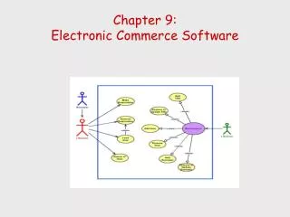
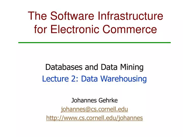
The Software Infrastructure for Electronic Commerce. Databases and Data Mining Lecture 2: Data Warehousing Johannes Gehrke johannes@cs.cornell.edu http://www.cs.cornell.edu/johannes. Overview. Conceptual design Querying relational data

E N D
The Software Infrastructurefor Electronic Commerce Databases and Data Mining Lecture 2: Data Warehousing Johannes Gehrke johannes@cs.cornell.edu http://www.cs.cornell.edu/johannes
Overview • Conceptual design • Querying relational data • Dimensional data modeling: OLTP versus decision support We will design and analyze a data mart with click-stream data as an illustrative example.
The Database Design Process • Requirement analysis • Conceptual design using the entity-relationship (ER) model • Schema refinement • Normalization • Physical tuning
Overview of Database Design • Conceptual design: (ER Model is used at this stage.) • What are the entities and relationships in the enterprise? • What information about these entities and relationships should we store in the database? • What are the integrity constraints or business rules that hold? • A database `schema’ in the ER Model can be represented pictorially (ER diagrams). • Can map an ER diagram into a relational schema.
name ssn lot Employees ER Model Basics • Entity:Real-world object distinguishable fromother objects. Anentity is described (inDB) using a set of attributes. • Entity Set: A collection of similar entities. E.g., all employees. • All entities in an entity set have the same set of attributes. • Each entity set has a key. • Each attribute has a domain.
ER Model Basics (Contd.) • Relationship: Association among two or more entities. E.g., Johannes works in the computer science department. • Relationship set: Collection of similar relationships. since name dname ssn budget lot did Works_In Employees Departments
An n-ary relationship set R relates n entity sets E1 ... En; each relationship in R involves entitiese1, ..., en Same entity set could participate in different relationship sets, or in different “roles” in same set. ER-Model Basics (Contd.) name ssn address Employees subor-dinate super-visor Reports_To
since name dname ssn lot Employees Manages Key Constraints • Consider Works_In: An employee can work in many departments; a department can have many employees. • In contrast, each deptartment has at most one manager, according to the key constraint on Manages. did budget Departments
Key Constraints (Contd.) • Several types of key-constraints: 1-to-1 1-to Many Many-to-1 Many-to-Many
Key constraints: Examples • Example Scenario 1: An inventory database contains information about parts and manufacturers. Each part is constructed by exactly one manufacturer. • Example Scenario 2: A customer database contains information about customers and sales persons. Each customer has exactly one primary sales person. • What do the ER diagrams look like?
Participation Constraints Does every department have a manager? If so, this is a participation constraint: The participation of Departments in Manages is said to be total (vs. partial). (Compare with foreign key constraints.) since since name name dname dname ssn did did budget budget lot Departments Employees Manages Works_In since
Participation Constraints: Examples • Example Scenario 1 (Contd.): Each part is constructed by exactly one manufacturer. • Example Scenario 2: Each customer has exactly one primary sales person.
ER Modeling: Case Study Drugwarehouse.com has offered you a free life-time supply of prescription drugs (no questions asked) if you design its database schema. Given the rising cost of health care, you agree. Here is the information that you gathered: • Patients are identified by their SSN, and we also store their names and age. • Doctors are identified by their SSN, and we also store their names and specialty. • Each patient has one primary care physician, and we want to know since when the patient has been with her primary care physician. • Each doctor has at least one patient.
ER Modeling: Summary • After the requirement analysis, the conceptual design develops a high-level description of the data • Main components: • Entities • Relationships • Attributes • Integrity constraints: Key constraints and participation constraints • We covered only a subset
Querying Relational Databases • “The” relational query language: SQL
Structured Query Language SELECT target-list FROM relation-list WHERE qualifications • relation-list: A list of relation names • target-list: A list of attributes of relations in relation-list • qualification: Comparisons (Attr op const or Attr1 op Attr2, where op is one of <,>,=,<=,>=,<>) combined using AND, OR and NOT.
Recall: Customer Relation • Relation schema:Customers(cid: integer, name: string, byear: integer, state: string) • Relation instance:
Example Schema:Customers( cid: integer, name: string, byear: integer, state: string) Query:SELECT Customers.cid, Customers.name, Customers.byear, Customers.stateFROM CustomersWHERE cid = 1950 Example Query
SELECTCustomers.cid, Customers.name,Customers.byear, Customers.state FROM Customers WHERE cid = 1960 Example Query
SELECTCustomers.cid, Customers.name,Customers.byear, Customers.state FROM Customers C WHERE cid = 1960 Range Variables
Example Query A range variable is a substitute for a relation name. • Query:SELECT C.cid, C.nameFROM Customers CWHERE C.byear = 1960
“*” is a shortcut for all fields Query:SELECT *FROM Customers CWHERE C.name=“Smith” Common Shortcuts
SELECT C.state FROM Customers C Example Query
DISTINCT Keyword DISTINCT:Eliminates duplicates in the output Query:SELECT DISTINCT C.stateFROM Customers C
Example Query • Query:SELECT C.cid, C.name, C.byear, C.stateFROM Customers CWHERE C.name=“Smith” • Answer:
Selection Predicates • Query:SELECT C.cid, C.name, C.byear, C.stateFROM Customers CWHERE C.name=“Smith” AND C.state=“NY” • Answer:
Combining Relations: Joins SELECT P.pid, P.pname FROM Products P, Transactions T WHERE P.pid = T.tid AND T.tdate < “2/1/2000”
Query: “Find the names and ids of customers who have made purchases before February 1, 2000.” SQL: SELECT C.name, C.id FROM Customers C, Transactions T WHERE C.cid = T.cid ANDT.tdate < “2/1/2000” Example Query
Example Query • Query: “Find the names and ids of the customers who have purchased MS Office Pro.” • SQL:SELECT C.name, C.idFROM Customers C, Transactions T, Products P WHERE C.cid = T.cid AND T.pid = P.pid AND P.pname = “MS Office Pro”
Aggregate Operators • SQL allows computation of summary statistics for a collection of records. • Operators: • MAX (maximum value) • MIN (minimum value) • SUM • AVG (average) • COUNT (distinct number)
Example Queries • Query: “Tell me the minimum and maximum price of all products.” • SQL:SELECT MAX(P.price), MIN(P.price)FROM Products P • Query: “How many different products do we have?” • SQL:SELECT COUNT(*)FROM Products
GROUP BY and HAVING • Instead of applying aggregate operators to all (qualifying) tuples, apply aggregate operators to each of several groups of tuples. • Example: For each year, show the number of customers who are born that year. • Conceptually, many queries, one query per year. • Suppose we know that years are between 1900 and 2000, we can write 1001 queries that look like this:SELECT COUNT(*)FROM Customers CWHERE C.byear = i
Queries With GROUP BY and HAVING • Extended SQL Query Structure:SELECT [DISTINCT] target-listFROM relation-listWHERE tuple-qualificationGROUP BY grouping-listHAVING group-qualification
Example: GROUP BY • Example: For each year, show the number of customers who are born that year. • SQL:SELECT C.byear, COUNT(*)FROM Customers CGROUP BY C.byear
Example • Query: “For each customer, list the price of the most expensive product she purchased.” • SQL:SELECT C.cid, C.name, MAX(P.price)FROM Customers C, Transactions T, Products PWHERE C.cid = T.cid and T.pid = P.pidGROUP BY C.cid, C.name
Example • Query: “For each product that has been sold at least twice, output how often it has been sold so far.” • SQL:SELECT P.pid, P.pname, COUNT(*)FROM Products P, Transactions TWHERE P.pid = T.pidGROUP BY P.pid, P.pnameHAVING COUNT(*) > 1
Notes on GROUP BY and HAVING SELECT [DISTINCT] attribute-list, aggregate-listFROM relation-listWHERE record-qualificationGROUP BY grouping-listHAVING group-qualification • The query generates one output record per group. A group is a set of tuples that have the same value for all attributes in grouping-list.
Notes on GROUP BY and HAVING SELECT [DISTINCT] attribute-list, aggregate-listFROM relation-listWHERE record-qualificationGROUP BY grouping-listHAVING group-qualification • The attribute list must be a subset of the grouping-list. Why? Each answer record corresponds to a group, and there must be a single value per group. • The aggregate-list generates one value per group. • What about the group-qualification?
Summary: SQL • Powerful query language for relational database systems • End-users usually do not write SQL, but graphical user front-ends generate SQL queries • SQL completely isolates users from the physical structure of the DBMS You can tune your DBMS for performance and your applications do not change (This is physical data independence!)
From OLTP To The Data Warehouse • Traditionally, database systems stored data relevant to current business processes • Old data was archived or purged • Your database stores the current snapshot of your business: • Your current customers with current addresses • Your current inventory • Your current orders • My current account balance
The Data Warehouse • The data warehouse is a historical collection of all your data for analysis purposes • Examples: • Current customers versus all customers • Current orders versus history of all orders • Current inventory versus history of all shipments • Thus the data warehouse stores information that might be useless for the operational part of your business
Terminology • OLTP (Online Transaction Processing) • DSS (Decision Support System) • DW (Data Warehouse) • OLAP (Online Analytical Processing)
OLTP Architecture Clients OLTPDBMSs CashRegister Product Purchase Inventory Update
DW Architecture Clients Data Warehouse Server Information Sources OLAP Servers MOLAP OLTPDBMSs Analysis Query/Reporting ExtractCleanTransformAggregateLoadUpdate Other Data Sources Data Mining Data Marts ROLAP
The Data Warehouse Market • Market forecast for warehousing tools in 2002: $8 billion (IDC 7/1999) • Revenue forecast for data warehouse front-end tools:1998 $1.6 billion1999 $2.1 billion2000 $2.8 billion(Gartner Group 2/1999)
Dimensional Data Modeling • Recall: The relational model. The dimensional data model: • Relational model with two different types of attributes and tables. • Attribute level: Facts (numerical, additive, dependent) versus dimensions (descriptive, independent). • Table level: Fact tables (large tables with facts and foreign keys to dimensions) versus dimension tables (small tables with dimensions).
Fact (attribute): Measures performance of a business. Example facts: Sales, budget, profit, inventory Example fact table: Transactions (timekey, storekey, pkey, promkey, ckey, units, price) Dimension (attribute): Specifies a fact. Example dimension: Product, customer data, sales person, store Example dimension table: Customer (ckey, firstname, lastname, address, dateOfBirth, occupation, …) Dimensional Modeling (Contd.)
OLTP Regular relational schema Update queries change data in the database:One instance of a customer with a unique customerID Queries return information about the current state of affairs The data warehouse Dimensional model Update queries create new records in the database:Several instances of the same customer (with different data), in case the customer moved Queries return aggregate information about historical facts OLTP Versus The Data Warehouse
Example: Dimensional Data Modeling Customers: Dimension Table Time: Dim. Table Transactions: Fact Table Products: Dim. Table